3.3.3) The PIA SCP Window

The PIA SCP Window serves to control the processing from the SCP to the SPD level. It is reached via the button "Plot and Reduce Data" in the menu of the PIA Measurement Buffer Control Panel or it is automatically displayed when processing data from the PIA SRD Data Display Window. The maximum number of opened SCP Windows is restricted to two.

This chapter describes the PIA SCP Data Display window and directly associated sub-windows.

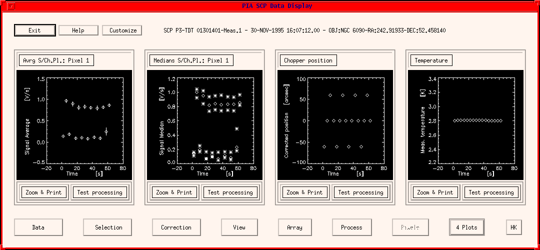
Basically, the SCP window (Figure 1) is divided into three rows:

• The upper row: It contains control buttons, main measurement information and in the case of a C100 or C200 measurement detector array pixel buttons.
• The middle row: It shows a number of plots (up to 4) and associated buttons, acting on the displayed plots or the data displayed in the corresponding plot.
• The lower row: It contains several data handling and processing buttons, acting on the whole measurement. It includes a button to chose the number of plots in the middle row.

---

FIGURE 1: The PIA SCP Window 

---

Remark on Upper and Middle Row:

Since the upper row and the middle row are very similar to those of the ERD Window, the user is referred to the ERD description with the following differences:

1. Menu Bar on top: The submenu offers the following possibilities:
• Signal Average per Chopper Plateau [Volt/sec]
• Signal Median per Chopper Plateau [Volt/sec]
• Signal/CP Flag
• Chopper Position [arcsec]
• Temperature [K]
• FCS1 electrical power [mW]
• FCS2 electrical power [mW]
• Time Key
• Raster Point ID
• Signal Average per Chopper Plateau / Open pixel [V/sec]
• Signal Median per Chopper Plateau / Open pixel [V/sec]
• Signal Average per Chopper Plateau / Resistor pixel [V/sec]
• Signal Median per Chopper Plateau / Resistor pixel [V/sec]

---

The lower row

Data

This menu bar calls a submenu with the following options:

• Load: This calls the window Please Select a Measurement in order to load a new measurement into the SCP window, activating it for plotting and reduction. The measurement which was displayed still remains in the buffer, but is deactivated from this window.
• Save:
• To SCP buffer: this option can be used for putting the modified data present on the window into the dynamical buffer, together with all the modifications. The same position in the buffer can be used, thus overwriting the data which entered the window, or a new position, creating a new measurement in the general buffer. This allows for a re-call of the corrected data in a later stage, opening again the SCP window.
• to PIA internal file: this calls Please Select a File for Writing window and asks a filename (and directory) under which the data shall be saved (a default name is proposed) in internal PIA format. This gives the possibility of saving several times the same measurement differently corrected, avoiding confusion (several versions in the case of VMS files) or overwriting (in the UNIX case).

If the associated Compact Status file with the appropriate filename is not found in the directory chosen for saving the file, then it will be automatically saved, also in internal format. This makes it possible to reload the data in a later session without loading the data from the FITS files.
• to FITS external file: this saves the measurement in FITS format under the default name into the actual save directory.
• Print Values: This calls a text window displaying the SCP results with the possibility of printing or storing the output on file.
• Show Data: This calls the Show Structures -Plot Curves Menu (s.3.4.4) for complete access to the measurement buffer, allowing for plots, correlations, etc.

Selection

This menu bar calls a submenu with the single option:

• Discard Chopper Plateaux: This calls the PIA Chopper Plateau Selection Window in order to enter which chopper plateaux shall be discarded.


After selection the plots of the SCP Window will be refreshed with the discarded chopper plateaux being marked by different symbols, depending on the plot symbol style. Note that the selection criteria chosen remain active for all further processing steps within a session until they are modified again.They particularly affect all the pixels of the array detectors. With this menu it is not possible to set the parameters individually for each pixel or group of pixels.

Correction

This menu bar calls a submenu for corrections to be applied to the measurement with the following options:

• Vignetting: This performs the vignetting correction for all the pixels which belong to the measurement. The vignetting information is taken from the standard CALG files P##VIGN.FITS.
• Dark Current Subtr (obsolete): This performs the subtraction of the dark current. It is taken from the standard CALG file PDARKCURR.FITS and can be performed either on the SRD or on the SCP level. Since a dependence of this value on the ISO orbital position at the time of measuring was found, the dark current subtraction should be performed using:
• Dark Current Subtr. (orbital dep.): Tables containing the dark currents depending on the ISO orbital position are used, which are taken from the standard CALG files P##DARKC.FITS, where ## stands for the detector identifiers.
• Signal losses in chopped measurements: This option is only active for subtracted chopped measurements (which have not been reduced using the default "Ramps Pattern" procedure) and corrects for the losses by a subtracted signal from chopping between two fluxes.
• Signal Linearization: This corrects for the dependence of the detector response on the applied flux illumination. See under chapter 5, "The Processing Algorithms", for details.
• Straylight subtraction: This applies only to FCS measurements. It performs the straylight subtraction for all the pixels which belong to the measurement.
• Baseline drift modelling: This option is active, if the measurement contains more than 5 chopper plateaux. A graphical determination of baseline drift factors, as described further below ("Baseline drift graphical modelling"), is hereby possible. As usual there is the possibility of testing from every individual window, under Testing. Please note that the correction is applied to the data only if started from this button, and not from the one for testing.

View

This menu bar calls a submenu for obtaining the following information:

• Header Info: displays FITS header information of the corresponding measurement (including logs of the corrections performed by PIA on the data).
• Compact Status: displays information on instrument configuration present on the Compact Status file of the corresponding measurement.
• Auxiliary Files:
• IS Report: Instrument Station report recorded during the on-line monitoring of the displayed measurement (entries in PISR-FITS files).
• OLP Report: information recorded during the off-line pipeline processing of the displayed measurement (entries in the POLR-FITS files).
• EOHA: Edited Observation History Attributes corresponding to the measurement.
• EOHI: Edited Observation History Information corresponding to the measurement.

• Statistics Info:
• Stability Stats: opens a text window and a Show Structures - Plot Curves Menu with the statistics from the stability analysis corresponding to the measurement (if applied).
• Drift modelling: Statistics from the signal drift modelling corresponding to the measurement (if applied).
• Slopes variation: Statistics from the signal slopes variation analysis corresponding to the measurement (if applied).

Array

This menu bar calls a submenu with additional features for array data. It offers the following options:

• Images: This allows the signal values of all array pixels (for C100, C200) to be viewed in one single plot or per raster point. In case of a raster or scanning mode the user is asked for the raster point and chopper plateau to be taken. A PIA XSurface Window is created.
• Spectra: This allows the signal values of all pixels (for PHT-S) to be viewed in one single plot per raster point. A PIA XPlot Window is created.
• Time evolution: This allows to view the signal values versus pixel number (for C100, C200 and PHT-S) in one single plot:
• Time Slices: Calls a PIA Xplot Window to plot histogram of signals versus pixel number for each time step (in different colors),
• 3D View: Calls a PIA XSurface Window to plot a 3D-histogram of signals versus pixel number and time step.

Process

This menu bar calls a submenu in order to process the whole measurement to the next level. The submenu offers the following possibilities:

• Power calibration (for on-sky measurements only) - There are five alternatives to transfer signals in [V/s] to fluxes in [Jy] and surface brightnesses in [MJy/sr]:
  
  
• Default Responses: standard values in the CALG files PRESPONSE.FITS (for P- and C-detectors) and PSPECAL.FITS (for PHT-S),
• Chopped SPRF (only for PHT-S): calibration performed using the dynamic calibration for PHT-S chopped measurements.
• Actual Responses: the actual response as calculated from an FCS measurement via the menu choice "Responsivity Calculation",
• Interpolate Responses: a response distribution is calculated from the interpolation between two FCS measurements (eg. mapping case),
• Absolute Photometry: This is for the case of a measurement of source chopped against the FCS (old absolute photometry mode).
  
  
After a selection the processing immediately starts and the result will be displayed in a new AAP window. Intermediate results in the conversion from SCP to AAP ([V] ->  [Jy]) on the SPD level (in Watts)  can be accessed on an SPD Window using the buffers manager. 


• Responsivity Calculation (for FCS measurements only): This serves to determine the actual response.


From an FCS measurement the responsivity per pixel will be calculated and the result is displayed. For comparison the default response is also displayed. It is then possible to chose between default, actual response from averages, and actual response from medians. 



• Background Subtraction: 
  
  
• within measurement: This applies only for chopped measurements source versus background.


First the chopper steps are plotted in a new PIA XPLOT Window. Then the PIA Background Subtraction Window (s.3.3.6) is created which asks for several operations. The background subtraction is performed within this new window and the result is present in the SCP buffer. 



• another measurement:


This calls the window Please Select a Measurement in order to select a background measurement. After selection the subtraction will immediately be performed and the result is present in the SCP buffer, as shown by a separate informative window.



NOTE: When returning to the SCP Window the background subtracted values are not automatically loaded into this window. It is necessary to load them explicitly via the menu button "Data" and "Load" (the new measurement name has the suffix "subtracted").
• Dark Current Measurement Subtraction: Allows for subtraction of a specific measurement to determine the dark current. The measurement must have been reduced to the SCP level beforehand.

 
• Straylight Measurement Subtraction: from an FCS calibration measurement a specific measurement to determine the straylight can be subtracted.

Note: Although every subtraction of another measurement yields the same results, independently of how it is declared, a subtraction should be performed according to its purpose, in order that the S/W can check for validity, avoiding certain operations which are futile (eg. subtracting a measurement of dark current after having applied dark current subtraction with default values) or giving warnings in case this is not considered the right method (eg. warning that dark current has been subtracted from a measurement while a straylight measurement subtraction is intended). PIA writes on every measurement header all the operations performed and uses these keywords for checks.

Pixels

This menu bar is active only for C100, C200 and PHT-S data, where several pixels are to be analyzed. It calls a submenu with the following options:

Individual Choice: This calls the PIA Display Choice window. For each display window the user can specify the pixel number whose signal will be plotted. After the selection the window will be refreshed with the plots for the new pixels chosen.

Serial Increment: This selects the next subsequent pixel to each of those shown. When pressing this button, in each window containing pixel N the signal corresponding to pixel N+1 will be plotted.

N Plots

This button allows the number N of plot windows shown in the middle row of the SCP window to be selected. After a selection the window will immediately be refreshed, containing N plots. Please note that this number will be used also for further main level windows.

HK

This button calls a submenu for accessing the Housekeeping Menu to display the Housekeeping data associated to this measurement, as contained in the corresponding GEHK FITS product.

---

The associated windows

The PIA Chopper Plateau Selection Window

Note: This Window is very similar to the PIA Read-Out Selection Window (and the PIA Signal Selection Window) and is described there (s. 3.3.1).

---

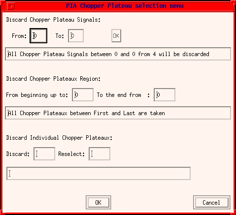
FIGURE 2: The PIA Selection Window 

---

The graphical modelling of baseline drifts:

Long term responsivity drifts are very difficult to model. A practical approach is to determine the correction factor by the eye-ball method.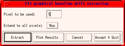

FIGURE 3: The PIA graphical baseline drift correction menu

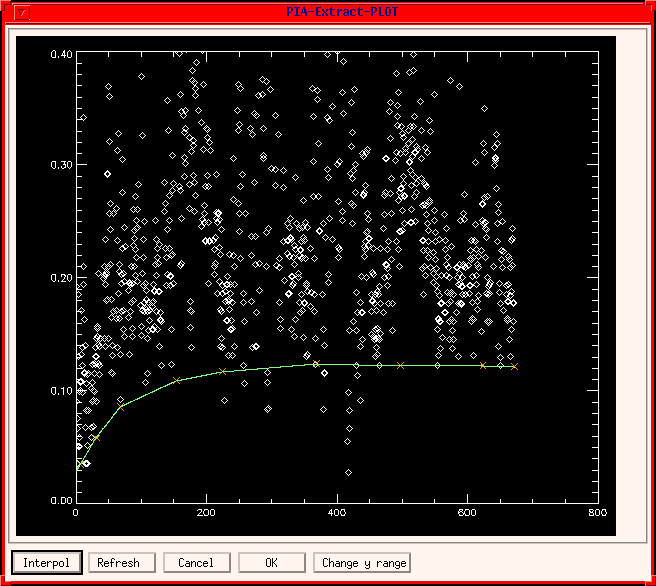
The main menu for baseline drift modelling is given by figure 3. It allows for choosing the detector pixel to be used. When starting only the buttons Extract and Cancel are active. Pushing the button Extract brings a special plot up. This plot, shown in Figure 4, allows the user to mark several points on it using the mouse, which are judged to correspond to the background baseline. In this example the plot corresponds to a P32 observation, which shows continuous background and source features. Once the points are marked they must be interpolated pushing the corresponding button. If the user is happy with the choice, he/she can accept & quit. A re-start is possible by using the Refresh button. If accepted, the results are passed to the main menu. The factors are normalized to the last point taken. The factors distribution can be extended to the other pixels of the sub-detector used (C100 in the example), or the other pixels can be individually treated (this is recommended).

---

 

Chapter history:

Date	Author	Description
16/05/1996	Martin Haas (MPIA)	First Version
06/06/1997	Carlos Gabriel (ESA/VILSPA - SAI)	Update (V6.3)
11/07/1997	Carlos Gabriel (ESA/VILSPA - SAI)	Update (V6.4)
13/10/1997	Carlos Gabriel (ESA/VILSPA - SAI)	Update (V6.5)
3/02/1998	Carlos Gabriel (ESA/VILSPA - SAI)	Update (V7.0)
23/08/1999	Carlos Gabriel (ESA/VILSPA - SAI)	Update (V8.0)