 |
Derive-SPDs' main input is Edited Raw Data (ERD), 24 Hz data containing detector readout (in bits) of the target's flux, of internal calibration exposures, of wavelength indicators, of dark currents and of housekeeping data. Within the ERD there is also information available from pointing or instrument status files. While processing, the pipeline software reads several Cal-G files.
For each detector, all data for one full reset interval are combined to a single current estimate at single wavelength and are then saved in the Standard Processed Data (SPD) file for that AOT. No attempt is made within Derive-SPD to average measurements of the same type (e.g. dark current measurements) on any time scale longer than one reset interval.
Each measurement for one reset interval of a given AOT is saved separately inside the same SPD product in chronological order of acquisition. The motivation for this is to offer to the observer the possibility of judging the stability and repeatability of SWS measurements. There is a one-to-one correspondence between AOTs and SPD files. That is, one AOT produces one SPD file.
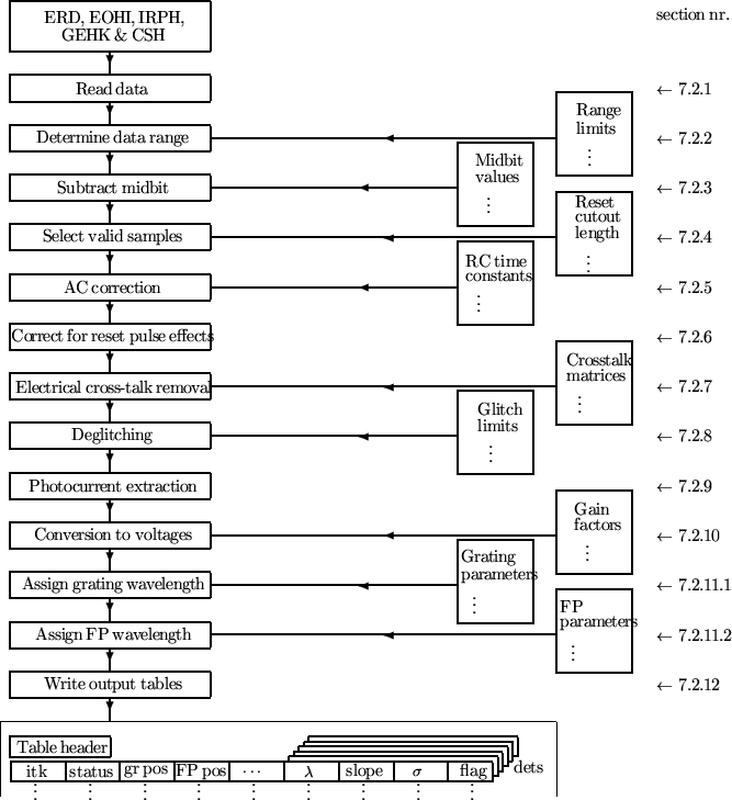
A basic overview of the Derive-SPD processing is given in Figure 7.1, the ERD and SPD files are described in Sections A.2.1 and A.3.1, and each step in the processing is described in the following sections.
The ERD data for the observation are read in. As discussed above, each AOT generates different types of data: astronomical measurements from the source, measurements of the currents for the grating and FP positions, measurements of the calibrators and dark currents. Each of these different types of data has a different physical meaning and serves a different purpose. Hence, the data must be flagged according to their type.
Each ERD data record is tagged with an Instrument Time Key (ITK) which points toward a unique record in the Compact Status History (CSH) file (see Section A.2.2). Cross-correlating the ERD ITK with the CSH, Executed Observation History per ICS (EOHI) and General Housekeeping (GEHK) files (both described in the ISO Handbook Volume I, [17]) allows a determination of the status of the SWS instrument at the time of the measurement and therefore of the type of the data recorded and the actual wavelength range covered.
The velocity of the spacecraft is obtained from the IRPH file. It is written into the header file and used later in the Derive-AAR processing stage.
Figure 7.2, top panel, shows 40 seconds of detector 16 ERD data from an SWS02 observation after reading in. This is the same SWS02 shown in Section 3.4.
This checks the data values and marks any out of limits. Values are OK when they are larger than 0 and less than 4095. Other data are flagged as out of limit. The values defining the ranges are kept in the calibration file Cal-G 4.
In SWS the detector readout voltages of between ![]() 10 and
10 and ![]() 10
V are converted
into a bit number ranging from 0 to 4095. The `midbit' is the bit value that
corresponds to 0 Volts. It is set to exactly half of 4095, i.e. 2047.5,
for all detectors. This data is stored in the calibration file Cal-G 2A.
10
V are converted
into a bit number ranging from 0 to 4095. The `midbit' is the bit value that
corresponds to 0 Volts. It is set to exactly half of 4095, i.e. 2047.5,
for all detectors. This data is stored in the calibration file Cal-G 2A.
The precise value of `midbit' is not important. It only determines the global level of the samples and also, due to later steps in the pipeline (Section 7.2.5), the overall level of the signal. This overall level is corrected again when subtracting the dark current (Section 7.3.3).
After each reset a number of samples should be ignored. They are too much affected by the reset pulse. This number is stored in the calibration file Cal-G 3. The values in the file are all set to 6 for OLP 10.
This is not formally a step in the DSPD processing as it is determined in each of the following steps what the valid samples are. It is presented here as henceforth all processing only affects the valid samples.
The amplifier chain contains a high pass filter. For a constant voltage gradient input the response of the amplifier is expected to asymptotically approach a constant value, i.e.
where ![]() is the output voltage at time
is the output voltage at time ![]() ,
, ![]() the input voltage
across the capacitor due to the accumulation of charges on the detector, and
the input voltage
across the capacitor due to the accumulation of charges on the detector, and
![]() the detector time constant. In order to later reconstruct the true
photo-current, it is first necessary to linearize the ramps, i.e. determine
the actual input voltages
the detector time constant. In order to later reconstruct the true
photo-current, it is first necessary to linearize the ramps, i.e. determine
the actual input voltages ![]() applied on the detector.
Each detector has its own time constant, which is stored in the calibration
file Cal-G 2.
applied on the detector.
Each detector has its own time constant, which is stored in the calibration
file Cal-G 2.
Knowing the RC time constant ![]() , it is straightforward to integrate
the above formula and derive the input voltage. The trapezium rule is
used to calculate the integral.
, it is straightforward to integrate
the above formula and derive the input voltage. The trapezium rule is
used to calculate the integral.
The time constants stored in Cal-G 2, however, are
expressed in terms of frequency, which relates to the ![]() in
Equation 7.2 as
in
Equation 7.2 as
![]() .
.
The second plot in Figure 7.2 shows 40 seconds of detector 16 after the determination of data range, `midbit' subtraction and correction for RC constant. The main difference between the first and second plot is due to this correction.
SWS defines the pulse-shape as the after-effect of the reset-pulse applied
after each reset interval. It manifests itself as an exponential curve with
typical decay times of 0.25 - 0.5 seconds and a typical amplitude of 20 - 50
![]() V. The pulse-shape is an additive component to the integrated signal
of the detector, while the impact on the observed ramp depends on the gain
setting of the instrument. Significant corrections are to be expected for
high gain observations only.
The pipeline corrects for the pulse-shape on an observation basis.
Consequently we do not rely on a fixed calibration file but use the data
itself to do the calibration.
V. The pulse-shape is an additive component to the integrated signal
of the detector, while the impact on the observed ramp depends on the gain
setting of the instrument. Significant corrections are to be expected for
high gain observations only.
The pipeline corrects for the pulse-shape on an observation basis.
Consequently we do not rely on a fixed calibration file but use the data
itself to do the calibration.
While the correction itself is a plain subtraction of the pulse-shape, the difficulty is to find the right pulse-shape. Per detector slopes are fitted to the readouts in each reset interval. The residuals contain the raw pulse-shape after-effects. To the residuals an exponential function is fitted, which determines the decay time for this detector in this observation. With this fixed decay time amplitudes of the exponential are determined, now for each reset interval individually. Subsequently the amplitudes are smoothed to reduce the noise and the resulting shapes are subtracted from the readouts.
More details of the method are explained in Lahuis 1998, [23] and Kester 2000, [20].
The third panel in Figure 7.2 shows 40 seconds of detector 16 after this processing step. Compared to the second panel the slopes have been straightened.
Due to parasitic capacitance between neighbouring detectors any signal in one grating detector will `leak' to other detectors (primarily the adjacent ones) in the same array. This `leak' to the adjacent detector is of the order of 10%.
Assuming the detector response is a linear function of the intensity of the
signal, a set of cross-talk matrices can be determined with constant correction
factors. The readouts ![]() of each individual detector
of each individual detector ![]() in the detector
array may then be corrected by applying the following formula:
in the detector
array may then be corrected by applying the following formula:
There is little effect on the data at this processing step, so a plot is not shown.
Glitches are sudden jumps in the output signal from a detector. How glitches are recognised in the data depends on which AOT the data is from. For SWS02, SWS06 and SWS07 the grating scanner does not move during a reset interval. Any sudden jump in the output of a detector during a reset interval is probably a glitch and can be recognised as such. For SWS01 however, the grating does move during a detector reset interval. It can scan across an entire line during a reset interval. If the line is strong enough there is a sudden increase in the signal level as the grating scans across it which might be mistaken for a glitch.
Therefore deglitching is handled differently in SWS01s compared to the other AOTs.
Glitches are recognized in the differentiated outputs of each detector,
![]() .
For each detector, the median,
.
For each detector, the median,
![]() median
median![]() , and the
median width,
, and the
median width,
![]() median
median![]() , of the
differentiated outputs are calculated.
A threshold is defined as
, of the
differentiated outputs are calculated.
A threshold is defined as
![]() , where
, where
![]() is a numerical factor and
is a numerical factor and ![]() is a minimum width. Both
of them are held in calibration file Cal-G 6. For OLP 10,
is a minimum width. Both
of them are held in calibration file Cal-G 6. For OLP 10, ![]() equals
8 and
equals
8 and ![]() equals 5.
Samples are flagged as glitched when
equals 5.
Samples are flagged as glitched when
![]() .
.
As a large fraction of all glitches is spread over more than one sample, the samples preceding and following them are checked again. If they are larger than 40% of the threshold, they are also marked as glitches.
In this processing step glitches are only marked as such. During the slope fitting (Section 7.2.9) a model including slope and glitches is fitted to all samples within the reset interval.
If glitches are detected during a reset this is noted in the flag word. Also the actual number of samples contributing to the slope calculation is decreased by the amount of glitched points found. This number appears in the offset tag (SWSPOFFS) in the SPD and in the tint tag (SWAATINT) in the AAR.
The SWS Glitch History (SWGH) file contains the two largest, if any, glitches found in each reset interval. For a description of this file see Section A.3.2.
The accuracy of deglitching depends not only on how well a glitch can be identified, but also on the effects of the glitch with time (the so called glitch-tails, see also Section 9.2.4). Especially in band 4 and in the FP bands glitch tails are occurring frequently. They show as a sudden increase of the flux decaying in about 10 seconds.
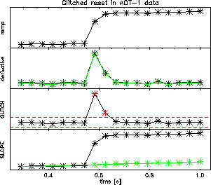
Figure 7.3 shows the effect of the deglitching software, showing the ERD and the SPD processed with and without the deglitching software. Where the software has not been used the glitches in the ERD cause the slope in the SPD to vary rapidly in time. Where the software has been used it has identified where the glitches occur, allowing them to be taken into account when calculating the slopes. The resultant SPD is much smoother.
For a further discussion of glitches and their correction see Kester 1999, [19], and Wieprecht, Wiezorrek & Haser 2000, [43].
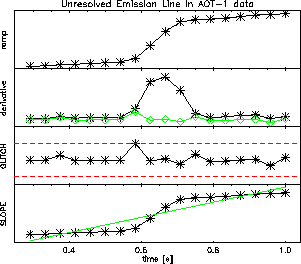
Because in SWS01s the grating is moving during a detector reset interval special care has to be taken reducing the data in order not to confuse narrow lines with glitches. In order to correctly distinguish between glitches and unresolved lines, a source signal is estimated and subtracted from the ramp derivative before deglitching is carried out. This source signal estimate is derived using the knowledge that the source signal should be constant while the grating scanner is not moving (as each detector only sees light in one wavelength). After this step the glitch detection is the same as in the other bands.
In SWS01s glitches are not only detected but also corrected with the stepsize found at the detected glitch position. An example of this glitch recognition technique is shown in Figure 7.4.
For more information on how glitches are recognised in SWS01 data see Lahuis, Kester & Shipman 2001, [24].


|
The net effect of this processing step is to convert the data from a set of 24 samples per second per detector to 1 point per reset interval per detector. Because of two schemes if glitch detection, also slope fitting come in two variants, one for SWS01 and one for the general case.
The current through the detector charges a capacitor. The voltage over the
capacitor is measured non-destructively during a reset interval. When
there is no glitch within the reset interval we can write the voltage, ![]() ,
as a linear function of the current,
,
as a linear function of the current, ![]() :
:
When one or more glitches are present during the interval we add a term
for each glitch. For a glitch at sample ![]() we have:
we have:
This model is fitted to the data ![]() by minimising
by minimising ![]() .
.
| (7.6) |
The error in the signal is obtained using the standard method to calculate the standard deviation in a slope:
The first factor in Equation 7.7 is the standard deviation of a linear model fit, and the second factor is the amount that has to be assigned to the slope part of the model.
The standard deviation is directly estimated from the fit residuals. Obviously, the accuracy depends not only on the intensity of the source, but also on how well the ramps have been previously linearized and therefore on the measurement error of the RC time constants, the pulse-shape correction and at high gain also digitization plays its role.
For band 3 detectors the slopes are multiplied by ![]() 1, as their bias is
reversed.
1, as their bias is
reversed.
Slope fitting in SWS01 is only different in the sense
that all detected glitches are corrected in the glitch detection part.
So there are no glitches to be fitted, no ![]() -functions. As the glitch
heights are estimated from the difference of two consecutive points
only, the fits and thus the slopes derived from them, are slightly less
efficient in the case where no flux change occurs during the reset
interval. It is a trade-off against grossly misfitting the slopes and
glitches in the presence of changing flux. In Kester 1999,
[19] a more precise method for doing the same is presented.
It takes much more time, however.
-functions. As the glitch
heights are estimated from the difference of two consecutive points
only, the fits and thus the slopes derived from them, are slightly less
efficient in the case where no flux change occurs during the reset
interval. It is a trade-off against grossly misfitting the slopes and
glitches in the presence of changing flux. In Kester 1999,
[19] a more precise method for doing the same is presented.
It takes much more time, however.
The electronics amplify the detector voltages with a preselected gain factor before the Analogue to Digital (AD) conversion. Each detector can be operated at three different gains of the amplifier chain. To convert the slopes to currents we have to undo the AD conversion and take into account the gains.
The current in ![]() V/s is related to the output of the AD converter,
in bits/s, by
V/s is related to the output of the AD converter,
in bits/s, by
| (7.8) |
The same conversion is applied to the standard deviations of Equation 7.7. These are stored in the stdev tag of the SPD (SWSPSTDV). These standard deviations are passed unchanged to the AAR (SWAASTDV), see Section 7.4.
The fourth plot in Figure 7.2 shows 40 seconds of
detector 16 after this processing step.
The data is now in ![]() V/s against time. All
that remains for Derive-SPD is to assign wavelengths to the individual data
points.
V/s against time. All
that remains for Derive-SPD is to assign wavelengths to the individual data
points.
All reset intervals of all detectors are assigned a wavelength within the limitations described below, even if the band was not requested or contains otherwise useless data. The wavelength is stored in the wave tag of the SPD (SWSPWAVE) or AAR (SWAAWAVE).
Within an ERD we have measurements, 24 times per second, of the grating position both for the SW and the LW sections of the grating. The grating position is measured in LVDT, see Section 3.2.1 and Chapter 4.
The grating positions are averaged over the valid samples within each reset interval and for each detector separately as the valid samples may differ from detector to detector. This results for SWS01s in potentially different values for the grating position for each detector. In all other AOTs the scanner does not move during a reset interval.
Subsequently the averaged grating positions are converted into grating
angles via the grating polynome. This is a 5th order polynome of which
the (time dependent) parameters are stored in the calibration file
Cal-G 16ET7.1.
The grating angle, ![]() , is used to obtain the wavelength,
, is used to obtain the wavelength, ![]() ,
via
,
via
![]() is the grating constant. It is taken from calibration file Cal-G 16C.
The angle
is the grating constant. It is taken from calibration file Cal-G 16C.
The angle ![]() runs from the optical axis
to the entrance slit. It is stored in the calibration file Cal-G 16A.
The angle
runs from the optical axis
to the entrance slit. It is stored in the calibration file Cal-G 16A.
The angle ![]() runs from the optical axis to the detector pixel. It
is stored in the calibration file Cal-G 16B.The spectral
order
runs from the optical axis to the detector pixel. It
is stored in the calibration file Cal-G 16B.The spectral
order ![]() is
determined by calculating all the orders that give wavelengths
consistent with the transmission limits of the aperture filters in
combination with the detection limits of the blocks (Table
2.1).
is
determined by calculating all the orders that give wavelengths
consistent with the transmission limits of the aperture filters in
combination with the detection limits of the blocks (Table
2.1).
A valid wavelength can be assigned only when one order fits the criterion. The order found is incorporated in the flag, which accompanies every flux in the SPD (or AAR), see Table A.7. When no order fits the criterion, a wavelength of 0 is assigned and no order flag bit is set. When multiple orders are found, the wavelength is given its first order value while the order flag bits are all set, resulting in a value of 7.
The transmission limits are stored in the calibration file Cal-G 24. The detection limits of the detector blocks are stored in the calibration file Cal-G 23.
The SPD has two more tags related to the (grating) wavelengths: grating position (SWSPGPOS) and grating angle (SWSPGANG). The position and angle of the first sample of each reset interval is stored in there. As explained above, for SWS01s these tags do not convert directly into the wavelengths quoted for each detector because of the movement of the scanner.
When determining the wavelength transmitted by the FPs, the grating wavelength must first be calculated as the LW grating section serves as order filter for the scanning FPs. Once the grating wavelength has been determined, calibration file Cal-G 12 is used to transform the nominal FP-position (an engineering parameter of no interest to the observer) into a FP-gap. This mechanical gap width is then corrected to get the optical gap width (using calibration file Cal-G 18). The wavelength which passes through the FP is the one of which a whole multiple fits exactly in two times the optical gap width.
The FP-position is stored in the SPD as SWSPFPOS and the FP-gap in SWSPFGAP. There is one more item in the SPD which is related to the FP, the FP-current (SWSPFCUR). It is computationally not related to the other FP items. Actually it is not used at all.
The data produced by the processing chain above is written out to the SPD and glitch list SWGH files. Each AOT results in one SPD file. For a definition of the SPD file see Section A.3.1. Note that the SPD file, like an ERD file, contains science data interleaved with dark current measurements, photometric checks etc.
An SPD record is produced for every reset interval. Complexities arise when the reset intervals for the SW and LW sections of the instrument are different, due to the instrumental setup required to obtain the required S/N ratios in the different halves of the instrument. In this case there will be one SPD record (containing data for all detectors) for each of the shorter reset intervals, with the SPD for the longer reset interval having its flag word set to `No data' for the records when it did not contain a reset (see Table A.7) and contains `0' in the flux -- this sometimes confuses plotting programmes. As an example, if the SW grating had a reset interval of 1 second and the LW one of 2 seconds, an SPD record would be produced every second. Every SPD record for the SW detectors (1-24) would contain valid data, while only every other record for the LW detectors would contain valid data, the others being marked as `No data'.
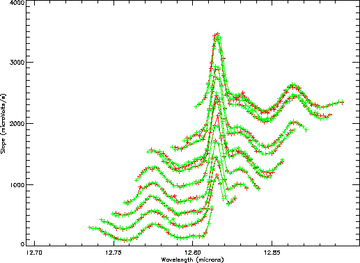
Figure 7.5 shows the final output of the Derive-SPD stage as detector output against wavelength.

|