Next: 7.7 Signal Processing: PHT32 Up: 7. Data Processing Level: Previous: 7.5 Signal Processing: Chopped

7.6.1 Obtaining the average signal per chopper plateau
- Ancillary data required:
7.6.2 Separation of source and background signal
7.6.3 Determine the signals averaged over a measurement
- 7.6.3.1 Rectangular mode
- 7.6.3.2 Sawtooth and Triangular mode
7.6.4 Spectral response function corrected for chopped signal losses
- Ancillary data required:
7.6.5 Determination of source and background spectrum
- Ancillary data required:

7.6 Signal Processing: Chopped PHT-S

In this section we first describe the extraction of the source signal from [source+background] and background signal. Subsequently the flux calibration for PHT-S is presented.

7.6.1 Obtaining the average signal per chopper plateau

Detailed description: none

The average signal per chopper plateau is obtained by applying processing steps 7.3.4 (deglitching), 7.3.5 (drift recognition), and 7.3.6 (mean signal per plateau).

Ancillary data required:

None

7.6.2 Separation of source and background signal

Detailed description: none

The background subtraction for a given chopper cycle and chopper mode is performed in this step.

For a given chopper cycle the background signal is subtracted from the [source+background] signal to obtain the source signal. This operation is repeated until the end of a measurement is encountered. Weighting factors are derived from the uncertainties which are used for the averaging of all chopper cycles at the end of a measurement.

In the following we describe the background subtraction method for the different chopper modes. Note that each cycle in triangular chopping mode consists of 4 plateaux referring to 2 [source+background] and 2 different background positions. In sawtooth mode there are 3 plateaux: 1 [source+background] and two different background positions. The following symbols are used for chopper cycle :

${s_{k}(x+b)_{1},~w_{k}(x+b)_{1}}$ : signal and weight of first [source+background] plateau;
${s_{k}(x+b)_{2},~w_{k}(x+b)_{2}}$ : signal and weight of second [source+background] plateau (triangular mode only);
${s_{k}(b1),~w_{k}(b1)}$ : signal and weight of the background at the first reference positiont;
${s_{k}(b2),~w_{k}(b2)}$ : signal and weight of the background at the second reference position;
${s_{k}(x+b),~w_{k}(x+b)}$ : average signal and weight from source plus background plateaux;
${s_{k}(x),~w_{k}(x)}$ : source signal and weight;
${s_{k}(b),~w_{k}(b)}$ : background signal and weight.

All signals are given in V/s, the weights are dimensionless.

7.6.2.1 Rectangular mode

Each cycle contains only 1 [source+background] plateau and 1 reference background position. For chopper cycle :

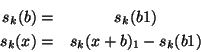
$\begin{eqnarray*} s_k(b) = & s_k(b1)\\ s_k(x) = & s_k(x+b)_1 - s_k(b1) \end{eqnarray*}$

The weighting factor is determined from the signal uncertainties:

$\begin{eqnarray*} w_k(u) = &\frac{1}{\sigma_k^{2}(u)}~~~{\rm for}~u=(x+b),\,b \... ...\frac{1} {\lbrack \sigma_k^{2}(x+b) + \sigma_k^{2}(b) \rbrack} \end{eqnarray*}$

where $\sigma_k(x+b)$ is the uncertainty in signal for the measurement on [source+background], etc.

7.6.2.2 Sawtooth mode

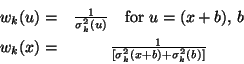
Each chopper cycle contains 1 [source+background] chopper plateau and 2 reference positions. For chopper cycle :

$\begin{eqnarray*} s_k(b) & = & \frac {s_k(b1) + s_k(b2)}{2}\\ s_k(x) & = & s_k(x+b) - s_k(b). \end{eqnarray*}$

With weighting factors:

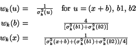
$\begin{eqnarray*} w_k(u) = & \frac{1}{\sigma_k^{2}(u)}~~~{\rm for}~u=(x+b),\,b1... ..._k^{2}(x+b) + (\sigma_k^{2}(b1) + \sigma_k^{2}(b2))/4 \rbrack} \end{eqnarray*}$

where $\sigma_{i}(x+b)$ is the uncertainty in the signal for the measurement on [source+background], etc.

7.6.2.3 Triangular mode

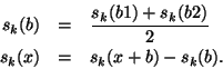
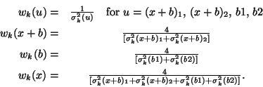
Each chopper cycle contains 2 [source+background] chopper plateaux and 2 reference positions. For chopper cycle :

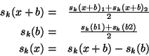
$\begin{eqnarray*} s_k(x+b) = & \frac {s_k(x+b)_{1} + s_k(x+b)_{2}}{2}\\ s_k(b... ...& \frac {s_k(b1) + s_k(b2)}{2}\\ s_k(x) = & s_k(x+b) - s_k(b) \end{eqnarray*}$

A weighting factor is also determined from the power uncertainties:

$\begin{eqnarray*} w_k(u) = & \frac{1}{\sigma_k^{2}(u)} ~~~{\rm for}~u=(x+b)_{1... ...k^{2}(x+b)_{2} + \sigma_k^{2}(b1) + \sigma_k^{2}(b2)\rbrack}. \end{eqnarray*}$

7.6.3 Determine the signals averaged over a measurement

Detailed description: none

The average source and background signals of all chopper cycles in a measurement is determined.

For all chopper cycles in a measurement, the weighted average is computed from the parameters per chopper cycle. For a given set of signals with weights obtained over a measurement, the weighted mean and its associated uncertainty $\sigma(s(X))$ is computed according to Equation 7.20. The mean can be either the signal of the source or background.

7.6.3.1 Rectangular mode

In rectangular mode the following mean signals are derived for each pixel:

$s(x)\pm\sigma(s(x))$ , $s(b)\pm\sigma(s(b))$ , and $s(x+b)\pm\sigma(s(x+b))$

7.6.3.2 Sawtooth and Triangular mode

In sawtooth and triangular mode the following mean signals are derived for each pixel:

$s(x)\pm\sigma(s(x))$ , $s(b)\pm\sigma(s(b))$ , $s(x+b)\pm\sigma(s(x+b))$ , $s(b1)\pm\sigma(s(b1))$ , and $s(b2)\pm\sigma(s(b2))$

7.6.4 Spectral response function corrected for chopped signal losses

Detailed description: Section 5.2.6

Analysis of chopped PHT-S data obtained from standard stars have shown that the PHT-S spectral response function is not unique but depends on the brightness of the source due to chopped signal losses. It is found that the amount of signal loss in a given detector pixel strongly depends on the source brightness in that pixel.

An accurate spectral response function for pixel is obtained by assuming an average spectral response function which is corrected per pixel for a source dependent signal loss:

$\begin{displaymath} C^{c,p}(i) = {\phi}(i)C^{c,p}_{ave}(i)~~~~~~{\rm [(V/s)/Jy]} \end{displaymath}$

(7.60)

with

$\begin{displaymath} {\phi}(i) = A^0(i) + A^1(i){\rm ^{10}log}(\vert s(x,i)\vert)~, \end{displaymath}$

(7.61)

where the superscripts refer to a chopped observation, and to a point source, and

$C^{c,p}(i)$ in (V/s)/Jy is the spectral response corrected for chopped signal loss for a given pixel ;
$C^{c,p}_{ave}(i)$ in (V/s)/Jy is the PHT-S average chopped spectral response function for a point source;
$\phi(i)$ is the signal dependent correction for the average spectral response function;
and (in ${\rm (^{10}log}(V/s))^{-1}$ ) are the coefficients for the signal dependent correction.

Ancillary data required:

The Cal-G file PSPECAL contains the average spectral response functions for both staring and chopped mode observations of point and extended sources, see Section 14.19.1. The file includes also the first order correction factors ( ).

7.6.5 Determination of source and background spectrum

Detailed description: none

The chopped PHT-S spectral energy distribution for the source and [source+background] is computed using the spectral response function corrected for chopper losses:

$\displaystyle F_{\nu}(x,i) =$	$\textstyle s(x,i)/C^{c,p}(i)~~~~{\rm [Jy]},$		(7.62)
$\displaystyle F_{\nu}(x+b,i) =$	$\textstyle s(x+b,i)/C^{c,p}(i)~~~~{\rm [Jy]},$		(7.63)

with

$\displaystyle {\Delta}F_{\nu}(x,i) =$	$\textstyle \sigma(s(x,i))/C^{c,p}(i)~~~~{\rm [Jy]}$		(7.64)
$\displaystyle {\Delta}F_{\nu}(x+b,i) =$	$\textstyle \sigma(s(x+b,i))/C^{c,p}(i)~~~~{\rm [Jy]}.$		(7.65)

The background spectrum is derived from the difference:

$\displaystyle F_{\nu}(b,i) =$	$\textstyle F_{\nu}(x+b,i)-F_{\nu}(x,i)~~~~{\rm [Jy]}$		(7.66)
$\displaystyle {\Delta}F_{\nu}(b,i) =$	$\textstyle \sqrt{{\Delta}F_{\nu}^2(x,i)+{\Delta}F_{\nu}^2(x+b,i)}~~~~{\rm [Jy]}.$		(7.67)

The resulting spectra are stored in the SPD products.

Ancillary data required:

none

Next: 7.7 Signal Processing: PHT32 Up: 7. Data Processing Level: Previous: 7.5 Signal Processing: Chopped

ISO Handbook Volume IV (PHT), Version 2.0.1, SAI/1999-069/Dc