


The strong source correction is described in Section 5.7.
To see if the strong
source correction needs to be applied to your data,
you should look at your LSAN data in ISAP:
this is best done by examining the overlapping
sub-spectra (in units of W cm![]()
![]() m
m![]() ) of detectors LW1-LW4
with their neighbours to see if their
spectral shapes agree. LW3 is the most non-linear detector so it is
best to check that one first. If some of the detectors do not agree on
spectral shape (and their spectra are `saggy') then the detector
sub-spectra are affected by non-linearity.
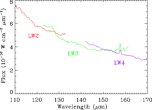
Figure 6.11 shows an
example of a strong source that has `saggy' sub-spectra and requires
the strong source correction. In particular you should check your data
for this if the saturated data flag comes up when data are loaded into ISAP.
) of detectors LW1-LW4
with their neighbours to see if their
spectral shapes agree. LW3 is the most non-linear detector so it is
best to check that one first. If some of the detectors do not agree on
spectral shape (and their spectra are `saggy') then the detector
sub-spectra are affected by non-linearity.
Figure 6.11 shows an
example of a strong source that has `saggy' sub-spectra and requires
the strong source correction. In particular you should check your data
for this if the saturated data flag comes up when data are loaded into ISAP.
A rough flux guide in Janskys:
for data with a flux of less than 500 Jy at 150 ![]() m the
correction will not be necessary (it is also unlikely that data in the
range of 500 to 1000 Jy will need the correction).
For data in the flux range of 1000 to 10000 Jy at 150
m the
correction will not be necessary (it is also unlikely that data in the
range of 500 to 1000 Jy will need the correction).
For data in the flux range of 1000 to 10000 Jy at 150 ![]() m
the correction might be required and the above steps should be followed for
further confirmation.
Above 10000 Jy it is very likely that the correction should be applied
to the data.
m
the correction might be required and the above steps should be followed for
further confirmation.
Above 10000 Jy it is very likely that the correction should be applied
to the data.
|
If any of your detector sub-spectra look saggy, the strong source correction needs to be applied to the data (the calibration of these saggy data is wrong, and cannot be trusted). The reason for, and the description of, the correction are exposed in Section 5.7.
If you have data requiring the strong source correction you can
contact the UK ISO Data Centre via isouk@rl.ac.uk. The
data will then be corrected by experts and the resulting data files
sent to you.
If you wish
to carry out the correction procedure yourself, you can use the SS_CORR
routine available in LIA (see Section 8.2.3), followed by the
SHORT_AAL procedure to process the corrected LSPD file into an
LSAN file.
The strong source correction has been made using Mars, as well as
Saturn. Both corrections should be applied to your data and you have to decide
which is best by looking at the agreement of the sub-spectra shapes
of the LSAN files.
In some cases the decision is not easy so if you require help in
deciding please contact isouk@rl.ac.uk for assistance.
The new LSAN and LSPD files can then be used in ISAP and LIA to do any further data reduction. On reading into ISAP you should see that the data are no longer saggy. You should not rely on the absolute fluxes of this LSAN file. The absolute calibration of the linear detectors can be trusted however and hence the sub-spectra of detectors LW1-LW4 can be scaled to one of these to produce a relative calibration. In doing this it should be seen that now the detectors agree on the shape of the spectrum.
Ideally the observations of strong sources were carried out using quarter-second ramps (integrations), however if they are half-second ramps the correction should not be applied directly to ramps of this length (see Section 5.8). You will need to contact isouk@rl.ac.uk to have your data processed as quarter-second ramps. Then the strong source correction will be carried out on the data (as described above) and all the relevant data files will be sent on.
In the near future, a table listing the observations that have already been corrected for strong-source effects will be available. The data from these corrected observations will be made available as 'Highly Processed Data Products' (HPDP) for download from the ISO Data Archive.