


Two dimensional raster and spatially oversampled mapping observations are processed to images in the equatorial (RA and Dec) coordinate system. For the construction of the images it is assumed that a detector footprint (or beam profile) can be represented by a simple `top-hat' function: the emission is 1 inside the detector area and zero outside. In addition, the circular apertures have perfectly circular footprints and the square PHT-P apertures and PHT-C detector pixels are considered to be perfectly square. The positions of each detector pixel per raster point have already been determined in the processing steps described in Section 8.3.3. This section describes the co-addition steps to obtain an image.
Note that in the remainder of this section a clear distinction should be made between detector pixel and image pixel, the former being one of the 9 (for C100) or 4 (for C200) elements in the detector array and the latter being a `picture element' of an image.
The mapping software yields three products:
Operation: Correct for possible flat-field patterns
Assessment of PHT22 or PHT32 maps have shown that there are systematic flat-field patterns of the C100 and the C200 arrays due to inconsistent surface brightness calibration of the individual detector pixels. The patterns are most prominent in maps with a poor overlap among the individual pixels.
To correct for these patterns a statistical flat-field was applied according to the following steps:
| (8.13) |
| (8.14) |
This correction is only applied if the raster map contains 20
or more raster steps for PHT22 raster maps or ![]() 20 chopper
plateaux for PHT32 maps.
The corrections
20 chopper
plateaux for PHT32 maps.
The corrections ![]() are written in the PGAI
product header
with keyword FFP
are written in the PGAI
product header
with keyword FFP![]() F
F![]() , where
, where ![]() is pixel number and
is pixel number and ![]() filter
number in AOT.
filter
number in AOT.
Operation: Define the size of the image pixel
The angular dimensions of an image pixel in OLP depend only on the detector subsystem used and is independent on the filter/aperture combination. The values are listed in Table 8.1.
| Detector | Shortest | Airy disc | Pixel |
| used | wavelength | diameter | size |
| [ |
[arcsec] | [arcsec] | |
| P1 | 3.2 | 2.8 | 8.0 |
| P2 | 20 | 17.7 | 8.0 |
| P3 | 60 | 50.3 | 8.0 |
| C100 | 70 (C_50) | 41.9 | 15.0 |
| C200 | 120 | 101.0 | 15.0 |
Based on the image pixel size, the fine-grid is defined to compute the fractional pixel coverage. The optimum fine-grid size in terms of realistic processing times has been decided to be:
| (8.15) |
Operation: Calculate the angular dimensions of the image required
to contain the full raster scan in equatorial coordinates.
The maximum size of the image is calculated using the following parameters:
The centre of the raster scan is defined as the image centre. The dimensions of the frame in equatorial coordinates are derived as follows. For all raster points (m,n) determine:
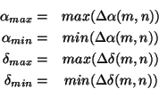
where:
The components
![]() and
and
![]() are computed
using spherical trigonometry.
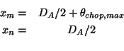
The margins around the raster grid is determined by D
are computed
using spherical trigonometry.
The margins around the raster grid is determined by D![]() and the
maximum chopper deflection
and the
maximum chopper deflection
![]() , in raster orientation:
, in raster orientation:
Then the map dimensions ![]() and
and ![]() are computed from:
are computed from:
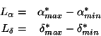
with
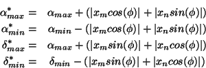
where ![]() is the spacecraft roll angle.
is the spacecraft roll angle.
The rectangular image frame is therefore chosen so large that the entire area covered by the detectors in the raster fits inside. Depending on the rotation angle of the raster as well as the sampling step sizes with respect to the size and rotation of the detector, undefined frame areas may be present.
The minimum number of image pixels required to map the whole of the raster
area is calculated from the dimensions of the raster and the image
pixel size ![]() , as follows:
, as follows:
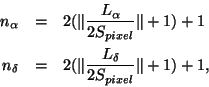
in which ![]() denotes `the integer value of' - i.e. the initial value is
rounded down to the nearest integer.
denotes `the integer value of' - i.e. the initial value is
rounded down to the nearest integer.
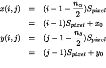
Also calculated at this stage are the angular coordinates of the image
pixel origin which is defined as the bottom left hand corner (blhc) of
image pixel ![]() .
.
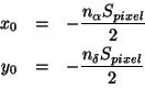
These are used subsequently to translate between the coordinate origin at the centre of the image and the origin of the pixel coordinates.
Finally, the angular coordinates of an image pixel (![]() ) are:
) are:
Operation: Map data from a given detector pixel, raster position,
and chopper offset combination onto the image.
We define a sky sample to be a sky observation for a given detector
pixel, at raster position (m,n), and chopper deflection
![]() .
A sky sample has a raster dwell time or chopper dwell time (in case
of PHT32 maps).
.
A sky sample has a raster dwell time or chopper dwell time (in case
of PHT32 maps).
The fine grid (Section 8.5.2) is used to determine the fractional coverage of the image pixel by the detector footprint. The fine-grid size is chosen such that it is a simple factor of the image pixel size: there is an integral number of grid points per image pixel.
Therefore for each sky sample the following steps are performed:
Operation: Accumulate the sky samples and derive
the average surface brightness, uncertainty and exposure.
The contribution from the ![]() sky sample to the mean brightness,
brightness uncertainty, and exposure time at image pixel
sky sample to the mean brightness,
brightness uncertainty, and exposure time at image pixel ![]() are denoted
are denoted
![]() ,
, ![]() and
and ![]() respectively.
The accumulated sums of the contributions from the first
respectively.
The accumulated sums of the contributions from the first ![]() pointings are denoted by
pointings are denoted by ![]() ,
, ![]() and
and ![]() .
.
The effective exposure time of sky sample ![]() at image pixel
at image pixel ![]() is
the fraction of the image pixel covered by the aperture for a given
sample multiplied by the plateau length (Section 8.3.2)
converted to seconds,
is
the fraction of the image pixel covered by the aperture for a given
sample multiplied by the plateau length (Section 8.3.2)
converted to seconds, ![]() :
:
| (8.16) |
To calculate the total exposure on the image pixel, the contributions from all sky samples are summed. The surface brightness values and the corresponding uncertainties are summed thereby using the exposure times as weights.
![\begin{eqnarray*}
E_{n+1}(i,j) = & E_{n}(i,j) + e_{n+1}(i,j)~~~~~~~{\rm [s]}\\ ...
...j) + e_{n+1}(i,j)u_{n+1}^{2}(i,j)
~~~~~~~{\rm [MJy\,sr^{-1}]}.
\end{eqnarray*}](img811.gif)
The accumulated sums for all sky samples
are used to derive images of total exposure time ![]() ,
mean brightness
,
mean brightness ![]() and brightness uncertainty
and brightness uncertainty ![]() .
.
![\begin{eqnarray*}
E_{total}(i,j) & = & E_{N}(i,j)\\
& = & \sum_{n=1}^{N} e_{n}(i,j)~~~~~~~{\rm [s]}
\end{eqnarray*}](img815.gif)
![\begin{eqnarray*}
{\overline B}(i,j) & = & B_{N}(i,j)/E_{N}(i,j)\\
& = & \fra...
...}}
\sum_{n=1}^{N} e_{n}(i,j)b_{n}
~~~~~~~{\rm [MJy\,sr^{-1}]}
\end{eqnarray*}](img816.gif)
![\begin{eqnarray*}
U_{rms}(i,j) & = & \left(\frac{1}{E_{N}} {U_{N}(i,j)}
\right...
...}^{2}(i,j)}
\right)^{\frac{1}{2}}
~~~~~~~{\rm [MJy\,sr^{-1}]}
\end{eqnarray*}](img817.gif)
Operation: Write a set of complete photometric image
products.
First write the product FITS header followed by the processed data in a primary array. The derived surface brightness (in MJy/sr), brightness uncertainty (in MJy/sr) and exposure time (in s) images are stored in separate products.
Detailed product descriptions can be found in Sections 13.4, 13.4.6 (product PGAI), 13.4.7 (product PGAU), and 13.4.8 (product PGAT) for the brightness, uncertainty and exposure time images.
Operation: Write a complete PHT-P raster photometry
product.
Write the product FITS header followed by the processed data in a binary table with each record containing the data for a single filter and sky position.
Detailed product descriptions can be found in Sections 13.4 and 13.4.9 (product PPAS).
Operation: Write a complete PHT-C raster photometry
product.
Write the product FITS header followed by the processed data in a binary table with each record containing the data for a single filter and sky position.
Detailed product descriptions can be found in Sections 13.4 and 13.4.10 (product PCAS).