The LWS photoconducting detectors usually drift upwards in responsivity
with time owing to the
impact of ambient ionising radiation. This drift in responsivity must be
corrected for before co-adding of individual scans. This is referred to as
the responsivity drift correction.
The absolute flux calibration on the other hand, involves
referring the responsivity of the detectors at the time of the observation
to the responsivity at the time of the calibrator (Uranus) observation.
This is referred
to as the absolute responsivity correction.
Both corrections make use of the response to a standard illuminator flash
sequence performed before and after each observation. The following sections
describe
how these corrections are performed.
From Version 7 of the pipeline onwards the responsivity drift correction was only performed for AOTs L01 and L03. This is because the correction did not work very sucessfully for L02 and L04 AOTs. The keyword LORELDN in the LSAN header indicates if the responsivity drift correction has been performed or not.
Before these corrections are applied, the data must be divided into `groups'. Each group will have a separate responsivity drift correction and absolute responsivity correction calculated and applied. The LGIF, group information file, contains one record for each group. The LGIF file identifies the start and end ITK of each group and also records information which is constant over the group. This includes the absolute responsivity and responsivity drift correction information for the group.
The grouping of data depends upon the AOT type. The easiest way of describing the grouping is to define the condition for the current group to end and a new group to start. A new group starts when:
For each group identified, a single reference time is calculated. This is the point at which the absolute responsivity correction will be calculated for the group. It is also the point where the responsivity drift correction will be normalised.
The reference time is simply half way between the time of the start and end of the group. This reference time is written into the LGIF file.
Processing of illuminator flashes
The first stage of the absolute responsivity correction is to process each illuminator flash in the observation. The aim is to find for each flash the ratio between the detector photocurrents from the flash and the reference photocurrents stored in the LCIR calibration file.
Only the `closed' illuminator flashes are used for the absolute responsivity correction. However, all illuminator flashes are first processed using the same method. The results of processing each flash are written into the LIAC file. This file contains one record for each flash in the observation.
The data for all illuminator flashes in each observation are read from the LIPD data file produced by SPL. This file contains the detector photocurrents for each ramp in each flash, plus the illuminator commanded status word and other information.
Background determination
The first stage of processing an illuminator flash is to determine the background photocurrent for each detector. These backgrounds will also be used in the dark current/straylight subtraction stage (see Section 4.4.2). The background value for each detector for each flash is written into the LIAC file.
The method for determining the background is as follows:
The uncertainty to be associated with
this value is given by
![]() for the set of averaged
photo currents. If there are less than three photo current
values then the maximum of the individual photo current uncertainties
is used.
for the set of averaged
photo currents. If there are less than three photo current
values then the maximum of the individual photo current uncertainties
is used.
Median clipping
The purpose of median clipping is to remove any outlying values from a set of measurements of the same value.
There must be at least five values for median clipping to be performed.
The method for median clipping is as follows:
Ratioing against reference data
For each illuminator flash a single absolute responsivity ratio is calculated for each detector. This is done by ratioing the photocurrents in the illuminator flash against reference flash data in the LCIR calibration file. The final ratio for each detector is written into the LIAC file.
The method for calculating the ratio for each detector depends on the kind of illuminator sequences performed in the observation. There was a major change in the on-board illuminator operations after ISO revolution 442. For all observations performed after revolution 442, the number of integrations performed for each illuminator were increased from 8 to 24.
Before revolution 442
Prior to ISO revolution 442 the removal of points affected
by glitches sometimes left just three or four points for an
individual illuminator, making it almost impossible to apply the OLP
Vesion 10
weighted-average method (see below).
Therefore, even in OLP Version 10,
these data are still processed using the 'OLP 8'
illuminator processing method.
This method
relies on using the point-by-point ratio of detector photocurrents
from the measured and references flashes.
The following sequence of
steps is performed:
Skip any photocurrent values which are set to zero in the LIPD file or the LCIR file. Skip any values for which the status word in the LCIR file indicates that it should be ignored.
If, while doing this, data are found to be missing from the LIPD file then jump to the start of the next illuminator level in the LIPD and LCIR files. Missing data are detected by a mismatch between the illuminator commanded status value in the LIPD and LCIR records. The warning message `LIMM' is issued each time this occurs. Data may be missing from the LIPD file because of telemetry dropouts or frame checksum errors. The LCIR file should not have any missing data.
After revolution 442 (the `OLP 10' method)
For observations performed after revolution 442, with the new illuminator scheme, the `OLP 10' method is used. It calculates the detector response correction factor using weighted-averages of the photocurrent ratios. The key processing steps are as follows:
These steps can be expressed in the following equations:
![\begin{displaymath}
R(d,j)=\frac{\sum_{i=1}^{5} \left[ \frac{r(d,i,j)}
{\sigma...
...
{\sum_{i=1}^{5} \left[ \frac{1}{\sigma_r(d,i,j)} \right]^2}
\end{displaymath}](img163.gif) |
(4.7) |
| (4.8) |
where ![]() and
and
![]() are the response correction factor
and standard deviation respectively for detector
are the response correction factor
and standard deviation respectively for detector ![]() ,
illuminator
,
illuminator ![]() and flash
and flash ![]() ;
; ![]() represents the weighted average of the response correction factor for detector
represents the weighted average of the response correction factor for detector
![]() and flash
and flash ![]() ; and
; and
![]() is the final response correction factor for detector
is the final response correction factor for detector ![]() after
averaging over the
after
averaging over the ![]() flashes in the observation.
flashes in the observation.
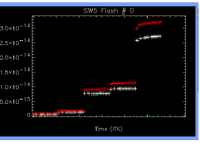
This method is expected to be an improvement on the `OLP 8' method because the response of the LWS detectors is known to be transient (Fouks 2001, [16] and Caux 2001, [5]), leading to a characteristic signature of the detector photocurrent for each illuminator as shown in Figure 4.4. In other words the scatter of photocurrent ratios for a given illuminator is not just pure statistical noise but is instead a systematic feature of the given detector.
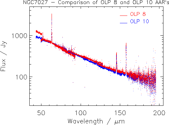
Figure 4.5 shows the spectrum of NGC 7027 respectively after application of both the `OLP 8' and `OLP 10' methods of illuminator processing. The level of continuity across the detectors in the `OLP 10' method can be clearly seen. Numerous other test cases and examples have confirmed the superiority of this method. We therefore conclude that the new illuminator processing method as implemented in OLP Version 10 is superior to the one in OLP Version 8 and leads to better stitched spectra. For off-axis point sources in the LWS beam or for extended sources, any residual discrepancy present between adjacent detectors, especially in the SW detectors, is most likely to be the result of the asymmetric LWS beam profile (Lloyd 2001, [28]).
Once all illuminator flashes have been processed the absolute responsivity can be derived.
For each group identified in the LGIF file the absolute responsivity ratio for each detector at the reference time is calculated. This is done using the data from the two closed illuminator flashes which surround the reference time. For each detector the absolute responsivity correction factor is calculated by doing a linear interpolation in time between the values at the two surrounding closed illuminator flashes. The uncertainty in this value is calculated as the highest of the uncertainties for the two surrounding values. The value of the correction factor and its uncertainty are written into the LGIF file.
The absolute responsivity correction is then performed on all of the science data within the group by subtracting the dark current from the detector photocurrent and then simply dividing the result by the absolute responsivity correction factor.
The responsivity drift correction corrects for the `drift' in responsivity during an observation. The drift is obtained from the information in the LSCA scan summary file. The responsivity drift is calculated separately for each group of data identified in the LGIF file.
The responsivity drift correction is only performed for AOTs L01 and L03. No drift correction is performed for AOTs L02 and L04.
Generation of LSCA, scan summary file
The LSCA scan summary file contains summary information for every scan in the observation. This includes a value which represents the signal level over the whole scan. This is calculated by finding the average signal per point in the scan. The signal values used are the values from the LSPD file, before any further processing. Any values which are marked as `invalid' in the LSAN status word are not included in this average.
For each scan a reference time is also calculated. This is simply the mid point between the times of the start and end of the scan.
Note that for L02 photometric observations no LSCA file is produced. This is because no responsivity drift correction is needed on this data. Also, since AAL regards each point in a photometric observation as a single scan, the LSCA file would be very large and would contain the same information as the LSAN file.
Determination of drift slope
For each group of data identified in the LGIF file a separate drift slope is calculated for each detector. The method is as follows:
Short scans are identified by comparing the total number of points (ramps) in each scan with the number of points in the first scan in the group. The first scan of a group is assumed to be a full scan. If the number of points in a scan is below half of the number in a full scan then it is classified as a short scan and discarded.
Note that the total number of ramps in a scan can also vary because of missing frames of telemetry data.
Note that in certain cases there may be insufficient valid data to determine
a drift slope. This can happen for the inactive detectors in FP observations.
The flag LGIFRSTA in the LGIF file indicates when this happens.
In this case no responsivity drift correction is performed.
Performing correction
Once the drift slopes have been calculated for each detector in each group the responsivity drift correction can be applied.
For each group identified in the LGIF file the corresponding flux data are corrected. The method for correction is as follows:
Each observation contains at least two `closed' illuminator flashes. During these illuminator flashes the wheel is set to an opaque position, removing the flux contributions due to the source. This is achieved by placing one of the FPs in the beam with the etalons misaligned. For grating observations, at least the first and last flashes in the observation will be closed flashes. For FP observations, all flashes are closed flashes since the FP is already in the beam and the etalons are misaligned before the illuminator flash is taken.
The background measurements during these closed illuminator flashes are a measure of the `dark signal' at the time they were taken. (The `dark signal' is the sum of the dark current and straylight). There is a separate background value for each detector. The values for the background measurements for the closed illuminator flashes are calculated using the information in the LIPD file. See Section 4.4.1 for details of how the background values are calculated. The backgrounds for each illuminator flash in the observation are written into the LIAC file. The closed illuminator flashes in the LIAC file are identified by the wheel absolute position field being set to either 0 (FPS) or 2 (FPL).
Between each pair of closed illuminator flashes in the observation a single dark current/straylight value is calculated for each detector. This is done by taking the mean of the two values from the surrounding flashes. The uncertainty in this value is given by the maximum of the two uncertainties from the surrounding flashes.
The dark current/straylight value is then subtracted from all of the detector photocurrent values between the pair of illuminator flashes. The uncertainty in the photocurrent is calculated by adding the uncertainties in the dark current/straylight and input photocurrent in quadrature. The dark current/straylight value subtracted from each scan is written into the scan summary file (LSCA). See Section 7.2.7.4 for details of the LSCA file.
From Version 8 onwards OLP uses a fixed dark current for processing of Fabry-Pérot data (AOTs L03 and L04). In OLP Version 10, for grating observations AAL checks each scan of each detector to see if the fixed dark current produces a better result (i.e. flux less negative) than the measured dark current. If this is the case then the fixed dark current is used instead of the measured dark current.
The values for this fixed dark current (one value per detector) have been determined as explained in Section 5.4 and are stored in the LCDK calibration file.
The grating mechanism positions are converted into wavelengths at this stage. The input to this stage is the grating measured positions (LVDT readouts) and the calibration information in the LCGW file (see Section 7.3.2 for a description of the LCGW file). The conversion is performed by means of an algorithm. The coefficients required for the algorithm are stored in the LCGW file.
It has been found that the relationship between LVDT and wavelength changed over time. The LCGW file therefore contains different coefficients for different time periods.
The wavelength conversion is performed in two steps. The first step is to
calculate the input beam angle to the grating, ![]() , for all ten
detectors. This is calculated using the following formula:
, for all ten
detectors. This is calculated using the following formula:
| (4.9) |
Where:
The input beam angle is then converted into wavelength for each detector by applying the grating equation and the geometry applicable to that detector. This is done using the following formula:
| (4.10) |
Where:
The efficiency of the LWS as a spectrometer varies with wavelength, mainly due to the bandpass filtering incorporated into each detector unit and the spectral response of the detector itself.
The Grating Relative Responsivity Wavelength Calibration file, LCGR (see Section 7.3.2), contains a spectrum of the relative response of the instrument in grating mode (The way the file is derived is described in Section 5.2). The wavelength for each point in the spectrum is looked up in this table and the corresponding responsivity value read. If no exact wavelength match is found within the table then a responsivity value is calculated by linear extrapolation between surrounding wavelength entries. The responsivity corrected flux then is calculated by dividing the flux by the responsivity value.
From OLP Version 7 the wavelength range in the LCGR file was extended compared to the previous versions. This is to allow for wavelength identification of features on overlapping detectors (See Figure 2.5). The relative photometric calibration at the edges of the range is very poor. Many detectors have a `steep sided' spectral response which makes the removal of the response uncertain. Also the steep sides enhance the effect of transient responses and the low throughput at the edges of the response curves leads to low signal-to-noise ratios. This region should therefore not be used for anything except wavelength identification of features. Data in this region can be identified by means of the `grating spectral responsivity warning' flag in the LSAN status word (see Section 7.2.8). When this warning flag is set this indicates that the data point has poor calibration and should not be used for anything other than wavelength identification. The wavelength ranges for which the LCGR calibration is nominal are also specified by keywords in the LCGR header (see Section 7.3.2.)
This correction only concerns grating scans. (For the corresponding correction for the FPs, see Section 4.4.7.)
The LCGB calibration file contains the spectral element size and uncertainty for each of the ten detectors. Auto-Analysis simply divides the flux for each detector by the appropriate spectral element size to perform the correction. The new flux uncertainty is calculated using the standard error formula.
The values of the spectral element sizes and uncertainties are written as keywords into the header of the LSAN file. Keywords LCGBddd contain the spectral element size for detector ddd (ddd='SW1'...'LW5'), while keywords LCGBUddd contain the corresponding uncertainties.
The wavelength calibration of a FP scan is done using a parametrised algorithm for the FP wavelength calibration. The wavelength calibration for FP spectra is done as follows:
| (4.11) |
where ![]() is the gap of the FP etalons,
is the gap of the FP etalons, ![]() is the FP position
value (as stored in the SPD product file (see
Section 7.2.5), and
is the FP position
value (as stored in the SPD product file (see
Section 7.2.5), and ![]() ,
, ![]() ,
, ![]() and
and
![]() are the FP wavelength calibration parameters read from
calibration file LCFW (see Section 7.3.2).
are the FP wavelength calibration parameters read from
calibration file LCFW (see Section 7.3.2).
| (4.12) |
where ![]() is the order of the scan,
is the order of the scan, ![]() is the gap of the FP
etalons and
is the gap of the FP
etalons and ![]() is the wavelength. INT means the integer
part of this division.
is the wavelength. INT means the integer
part of this division.
| (4.13) |
From OLP Version 8 onwards, the FP spectral responsivity calibration
has been replaced by the FP `throughput' correction, which is the
product of the FP
transmission multiplied by the FP resolution element. The method of
calibrating the total throughput of the FP's has been devised using Mars as
a calibration standard. This method uses a fitted polynomial between
the wavelength and the FP throughput and the results are FP fluxes
in units of W cm![]()
![]() m
m![]() .
.
The grating spectral responsivity calibration, described in Section 4.4.4, is also applied to FP data.
The wavelengths calculated in the previous stages are corrected for the velocity of the spacecraft and earth towards the target. The header of the LSPD file contains keywords which specify this velocity at three points during the observation. These keywords are written by a subroutine written by ESA which is external to the LWS pipeline (TREFDOP1 to 3). The velocity at each mechanism position in a scan is calculated by interpolating in time between the three given values. A second order curve fit is used for the interpolation. Once calculated, the coefficients of this fit are written into the LSAN header as the keywords LVCOEFFn (n=0-2).
The wavelength at each mechanism position is then corrected using the following formula:
| (4.14) |
Where:
Up to OLP Version 7, the absolute responsivity and the responsivity drift corrections were determined at the end of AAL. Therefore at this stage, before these corrections, the results of the previous calibration steps were written into the first product file produced by Auto-Analysis, named LSNR. This file was identical in structure to the final LSAN file, apart from a few minor differences. This file was provided to give observers access to the data before the absolute responsivity correction and responsivity drift corrections were applied. In a few cases these corrections did not work sucessfully. The LSNR file provided an alternative product file for those cases. After OLP Version 8 the responsivity corrections are performed at the start of the pipeline.
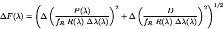
The LSAN file contains the field LSANFLXU which gives the estimation of the systematic flux error. The calculation of the uncertainty is detailed below, for the grating (AOTs L01 and L02) and the Fabry-Pérot (AOTs L03 and L04).
The grating flux is given by:
| (4.15) |
We can write the associated uncertainty as:
 |
(4.17) |
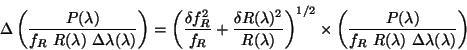 |
(4.18) |
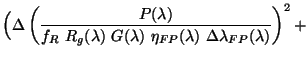
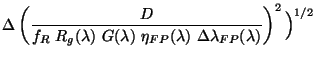
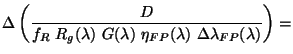
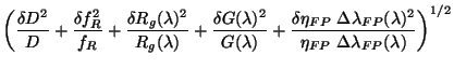
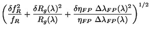
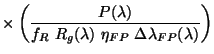
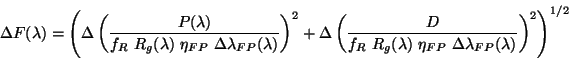
For the Fabry-Pérot the flux is given by:
| (4.19) |
 |
|||
 |
(4.20) |
 | |||
 |
|||
 |
(4.21) | ||
 | |||
|
|||
 |
(4.22) | ||
 | |||
 |
|||
 |
(4.23) | ||
All the terms except
![]() are known; this is calculated from a fit
to the error values in the original derivation of the
are known; this is calculated from a fit
to the error values in the original derivation of the
![]() parameters.
The absolute flux error placed in the LSAN.LSANFLXU tag is therefore:
parameters.
The absolute flux error placed in the LSAN.LSANFLXU tag is therefore:
 |
(4.24) |
Note that in this case also ![]() is set to zero in OLP Version 10
(see last paragraph of Section 4.4.10.1).
is set to zero in OLP Version 10
(see last paragraph of Section 4.4.10.1).