The transmission of optics and filters, as well as the quantum
efficiencies of the detectors exhibit non-flat spectral
dependencies. As a consequence, two sources radiating the
same power within a given wavelength range but with different spectral
shapes, produce two different signals. The flux density derived from
measurements of a source in a given filter has to be corrected for
this effect.
Therefore the flux density at the reference wavelength of a certain
filter of the broad-band photometry of ISOCAM
has been computed for an a priori assumed spectral shape, a
![]() law. This is the spectral density
distribution which has the same shape for
law. This is the spectral density
distribution which has the same shape for
![]() and
and
![]() , namely
, namely
![]() and
and
![]() . The same convention was adopted for the
flux densities quoted in the IRAS catalogues.
Although this is an arbitrary choice, this does not imply any loss
of generality, because the `real' flux density can be recovered by
the colour correction described hereafter.
In the CCG*WSPEC CAL-G files the spectral transmission curve
for each filter is given. The spectral transmission
. The same convention was adopted for the
flux densities quoted in the IRAS catalogues.
Although this is an arbitrary choice, this does not imply any loss
of generality, because the `real' flux density can be recovered by
the colour correction described hereafter.
In the CCG*WSPEC CAL-G files the spectral transmission curve
for each filter is given. The spectral transmission ![]() as defined for ISOCAM is the product of the filter transmission
as defined for ISOCAM is the product of the filter transmission
![]() and the detector quantum efficiency
and the detector quantum efficiency ![]() :
:
No transmission curve for the lenses has been included.
To determine the actual flux density one has to divide the
flux density
(derived after dividing the measured ADU/G/s by the SENSITIV parameter
of the CCG*WSPEC CAL-G files)
by the colour correction factor
![]() .
.
where
![]() is given by:
is given by:
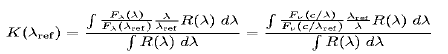 |
(A.1) |
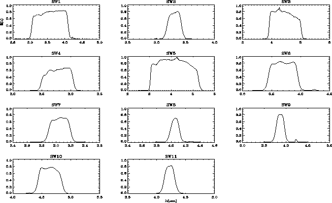
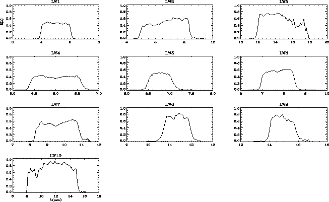
The spectral transmission ![]() of the SW and LW channels of
ISOCAM are shown in Figure A.1 and
Figure A.2, respectively. Colour corrections calculated
for different blackbody temperatures and for different power-laws (
of the SW and LW channels of
ISOCAM are shown in Figure A.1 and
Figure A.2, respectively. Colour corrections calculated
for different blackbody temperatures and for different power-laws (
![]() ) are shown in Tables A.1 -
A.4.
) are shown in Tables A.1 -
A.4.
| Temp | LW1 | LW2 | LW3 | LW4 | LW5 | LW6 | LW7 | LW8 | LW9 | LW10 |
| 10000 | 1.03 | 1.08 | 1.03 | 1.02 | 1.01 | 1.02 | 1.01 | 1.00 | 1.01 | 1.29 |
| 5000 | 1.02 | 1.07 | 1.03 | 1.02 | 1.01 | 1.00 | 1.01 | 1.00 | 1.01 | 1.27 |
| 4000 | 1.02 | 1.06 | 1.02 | 1.01 | 1.01 | 1.00 | 1.01 | 1.00 | 1.01 | 1.27 |
| 3000 | 1.02 | 1.05 | 1.03 | 1.01 | 1.01 | 1.00 | 1.01 | 1.00 | 1.01 | 1.26 |
| 2000 | 1.01 | 1.04 | 1.02 | 1.01 | 1.01 | 1.00 | 1.01 | 1.00 | 1.00 | 1.23 |
| 1000 | 1.00 | 0.99 | 1.01 | 1.00 | 1.00 | 0.99 | 1.00 | 1.00 | 1.00 | 1.17 |
| 800 | 0.99 | 0.98 | 1.01 | 1.00 | 1.00 | 0.99 | 1.00 | 1.00 | 1.00 | 1.13 |
| 600 | 0.99 | 0.96 | 1.00 | 0.99 | 1.00 | 0.99 | 0.99 | 1.00 | 1.00 | 1.08 |
| 400 | 1.01 | 0.98 | 0.99 | 1.00 | 1.00 | 1.00 | 0.99 | 1.00 | 1.00 | 1.00 |
| 300 | 1.06 | 1.06 | 0.98 | 1.01 | 1.00 | 1.01 | 0.99 | 1.00 | 1.00 | 0.94 |
| 250 | 1.12 | 1.17 | 0.98 | 1.04 | 1.00 | 1.03 | 1.00 | 1.00 | 1.00 | 0.91 |
| 200 | 1.26 | 1.43 | 0.99 | 1.09 | 1.00 | 1.06 | 1.03 | 1.00 | 1.00 | 0.91 |
| 150 | 1.65 | 2.18 | 1.02 | 1.24 | 1.02 | 1.16 | 1.11 | 1.02 | 1.00 | 0.96 |
| 100 | 3.30 | 6.23 | 1.20 | 1.78 | 1.09 | 1.51 | 1.42 | 1.06 | 1.02 | 1.30 |
|
|
LW1 | LW2 | LW3 | LW4 | LW5 | LW6 | LW7 | LW8 | LW9 | LW10 |
| 3.0 | 1.05 | 1.17 | 1.07 | 1.03 | 1.01 | 1.01 | 1.03 | 1.00 | 1.01 | 1.50 |
| 2.5 | 1.04 | 1.12 | 1.05 | 1.03 | 1.01 | 1.01 | 1.02 | 1.00 | 1.01 | 1.39 |
| 2.0 | 1.03 | 1.09 | 1.03 | 1.02 | 1.01 | 1.00 | 1.01 | 1.00 | 1.01 | 1.30 |
| 1.5 | 1.02 | 1.05 | 1.02 | 1.01 | 1.01 | 1.00 | 1.01 | 1.00 | 1.00 | 1.22 |
| 1.0 | 1.01 | 1.03 | 1.01 | 1.01 | 1.01 | 1.00 | 1.00 | 1.00 | 1.00 | 1.15 |
| 0.5 | 1.01 | 1.01 | 1.00 | 1.01 | 1.00 | 1.00 | 1.00 | 1.00 | 1.00 | 1.10 |
| 0.0 | 1.01 | 1.00 | 1.00 | 1.00 | 1.00 | 1.00 | 1.00 | 1.00 | 1.00 | 1.06 |
|
|
1.00 | 1.00 | 1.00 | 1.00 | 1.00 | 1.00 | 1.00 | 1.00 | 1.00 | 1.02 |
|
|
1.00 | 1.00 | 1.00 | 1.00 | 1.00 | 1.00 | 1.00 | 1.00 | 1.00 | 1.00 |
|
|
1.00 | 1.01 | 1.01 | 1.00 | 1.00 | 1.00 | 1.00 | 1.00 | 1.00 | 0.98 |
|
|
1.00 | 1.02 | 1.01 | 1.00 | 1.00 | 1.01 | 1.01 | 1.00 | 1.00 | 0.97 |
|
|
1.00 | 1.04 | 1.02 | 1.00 | 1.00 | 1.01 | 1.01 | 1.00 | 1.00 | 0.97 |
|
|
1.00 | 1.06 | 1.04 | 1.01 | 1.00 | 1.02 | 1.02 | 1.01 | 1.00 | 0.97 |
| Temp | SW1 | SW2 | SW3 | SW4 | SW5 | SW6 | SW7 | SW8 | SW9 | SW10 | SW11 |
| 10000 | 1.05 | 1.00 | 1.07 | 1.03 | 1.04 | 1.01 | 0.96 | 1.00 | 1.02 | 0.98 | 1.03 |
| 5000 | 1.04 | 1.00 | 1.06 | 1.03 | 1.02 | 1.01 | 0.97 | 1.00 | 1.02 | 0.99 | 1.03 |
| 4000 | 1.04 | 1.00 | 1.06 | 1.03 | 1.02 | 1.01 | 0.97 | 1.00 | 1.02 | 0.99 | 1.02 |
| 3000 | 1.03 | 1.00 | 1.05 | 1.02 | 1.01 | 1.00 | 0.97 | 1.00 | 1.02 | 0.99 | 1.02 |
| 2000 | 1.02 | 1.00 | 1.04 | 1.01 | 0.99 | 1.00 | 0.98 | 1.00 | 1.01 | 0.99 | 1.02 |
| 1000 | 0.99 | 1.00 | 1.00 | 0.98 | 0.96 | 1.00 | 1.01 | 1.00 | 1.00 | 0.99 | 1.00 |
| 800 | 0.98 | 1.00 | 0.99 | 0.98 | 0.97 | 1.00 | 1.03 | 1.00 | 0.99 | 1.00 | 1.00 |
| 600 | 0.99 | 1.01 | 0.97 | 0.98 | 1.01 | 1.00 | 1.06 | 1.00 | 0.99 | 1.01 | 0.99 |
| 400 | 1.06 | 1.02 | 0.96 | 1.04 | 1.27 | 1.02 | 1.15 | 1.01 | 0.97 | 1.03 | 0.96 |
| 300 | 1.21 | 1.05 | 0.97 | 1.14 | 1.80 | 1.06 | 1.26 | 1.01 | 0.97 | 1.06 | 0.94 |
| 250 | 1.40 | 1.07 | 1.01 | 1.27 | 2.53 | 1.11 | 1.38 | 1.02 | 0.97 | 1.08 | 0.93 |
| 200 | 1.84 | 1.12 | 1.11 | 1.56 | 4.53 | 1.22 | 1.59 | 1.03 | 0.98 | 1.14 | 0.92 |
| 150 | 3.23 | 1.25 | 1.39 | 2.36 | 13.54 | 1.50 | 2.10 | 1.06 | 1.03 | 1.24 | 0.91 |
| 100 | 13.52 | 1.66 | 2.68 | 6.54 | - | 2.78 | 4.17 | 1.16 | 1.39 | 1.59 | 0.91 |
|
|
SW1 | SW2 | SW3 | SW4 | SW5 | SW6 | SW7 | SW8 | SW9 | SW10 | SW11 |
| 3.0 | 1.09 | 1.00 | 1.11 | 1.06 | 1.12 | 1.02 | 0.95 | 1.00 | 1.03 | 0.98 | 1.04 |
| 2.5 | 1.07 | 1.00 | 1.09 | 1.05 | 1.08 | 1.01 | 0.96 | 1.00 | 1.03 | 0.98 | 1.03 |
| 2.0 | 1.06 | 1.00 | 1.08 | 1.04 | 1.05 | 1.01 | 0.96 | 1.00 | 1.02 | 0.98 | 1.03 |
| 1.5 | 1.04 | 1.00 | 1.06 | 1.03 | 1.03 | 1.01 | 0.97 | 1.00 | 1.02 | 0.99 | 1.02 |
| 1.0 | 1.03 | 1.00 | 1.04 | 1.02 | 1.01 | 1.00 | 0.97 | 1.00 | 1.01 | 0.99 | 1.02 |
| 0.5 | 1.02 | 1.00 | 1.03 | 1.02 | 1.00 | 1.00 | 0.98 | 1.00 | 1.01 | 0.99 | 1.01 |
| 0.0 | 1.01 | 1.00 | 1.02 | 1.01 | 0.99 | 1.00 | 0.99 | 1.00 | 1.01 | 0.99 | 1.01 |
|
|
1.00 | 1.00 | 1.01 | 1.00 | 0.99 | 1.00 | 0.99 | 1.00 | 1.00 | 1.00 | 1.00 |
|
|
1.00 | 1.00 | 1.00 | 1.00 | 1.00 | 1.00 | 1.00 | 1.00 | 1.00 | 1.00 | 1.00 |
|
|
1.00 | 1.00 | 0.99 | 1.00 | 1.01 | 1.00 | 1.01 | 1.00 | 1.00 | 1.00 | 1.00 |
|
|
1.00 | 1.00 | 0.99 | 0.99 | 1.03 | 1.00 | 1.01 | 1.00 | 0.99 | 1.01 | 0.99 |
|
|
1.00 | 1.00 | 0.98 | 0.99 | 1.06 | 1.00 | 1.02 | 1.00 | 0.99 | 1.01 | 0.99 |
|
|
1.00 | 1.00 | 0.98 | 0.99 | 1.09 | 1.00 | 1.03 | 1.00 | 0.99 | 1.02 | 0.98 |