


In order to derive flux density values (monochromatic fluxes) from measured in-band powers the following corrections and calibrations have to be done:
The latter correction contains the determination of the relative contribution of the flux density at the central wavelength of the band to the total flux in the band, depending on the assumed spectral shape of the source. Doing this calculation for a variety of source spectra and computing the ratios provides the colour correction factors between the various SEDs.
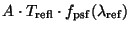
The flux conversion can be written in the following form:
| (C.2) |
where:
   = in-band power (unit: W)

   = reflection losses on optical elements

   = primary mirror area

   = wavelength dependent beam profile function

   = flux density of source at specific wavelength

   = system response at specific wavelength
Currently the in-band power calculation contains some simplification, in particular related to the beam profiles.
For point source fluxes the following calculation is done:
| (C.3) |
where:
= fraction of the point spread function at the reference wavelength

inside the aperture or pixelCal-G file PPPSF
For extended source fluxes the corresponding calculation is done:
| (C.4) |
where:
   = central obscuration factor by the secondary mirror

   = solid angle of selected aperture or pixel
In order to derive the flux density for the central wavelength, or more general a reference wavelength, of the bandpass the spectral energy distribution function is normalised with respect to the flux density at this wavelength:
| (C.5) |
where:
= flux density at reference wavelength
= functional dependence of spectral energy distribution of source with wavelength
Furthermore, for conversion between frequency range and wavelength range the following convention is used:
| (C.6) |
where:
m
)
= flux density in frequency range (unit: Wm
Hz
Solving this equation for ![]() yields:
yields:
| (C.7) |
where:
= speed of light
Using the normalisation with respect to the flux density value at the
reference wavelength and the convention for conversion of ![]() into
into
![]() the above formula of the in-band power can be solved for
the above formula of the in-band power can be solved for ![]() for a general source energy distribution
for a general source energy distribution ![]() :
:
| (C.8) |
where:
=
In the formula for the flux density ![]() the term, which is
dependent on the shape of the spectral energy distribution of the source,
is called the flux density conversion factor
the term, which is
dependent on the shape of the spectral energy distribution of the source,
is called the flux density conversion factor ![]()
| (C.9) |
In the following the conversion factors for specific SEDs are listed:
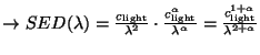
| (C.10) |
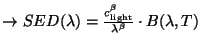 (
(| (C.11) |
Note that:
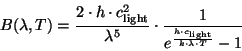 |
(C.12) |
where:
= Planck constant
= Boltzmann constant
B(correction factor from the frequency to wavelength conversion !
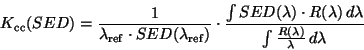
From the general formula of the colour correction in Appendix C.1 it follows that
| (C.13) |
and with the formulae from Appendix C.2.1 for
![]()
| (C.14) |
the colour correction factor is the ratio of the flux density conversion factors.
Inserting the formulae from Appendix C.2.2 for both flux density conversion factors this yields
 |
(C.15) |
In order to calculate the colour correction factors this needs a numerical
solution of the two integrals using the tabulated relative system response
![]() .
.