In the following we will address only some general aspects related to the in-orbit performance of the ISO detectors. More details are given in the corresponding instrument specific volumes (II to V) of the ISO Handbook.

5.6.1 Radiation effects

The performance of infrared detectors in space can be seriously affected by the ionising radiation environment. Charged particles can induce spikes (also known as `detector glitches'), higher dark current and detector noise as well as an increase level of responsivity.

The space radiation enviroment in which ISO was operated had four main constituents: geomagnetically trapped protons and electrons, solar protons and galactic cosmic rays (Nieminen 2001, [129]), each with a variable contribution depending both on the time of the mission and on the orbit phase.

The highly elliptic ISO orbit took the spacecraft deep into the Earth's radiation belts in its perigee ( $\sim$ 1000 km) and to the interplanetary space in its apogee ( $\sim$ 72000 km). To minimise the effect of charged particles impacting the ISO detectors at low altitudes, when the spacecraft crossed through the inner Van Allen belt (mainly composed of high-energy protons), the on-board instruments were switched off (see Section 4.2.2). At higher altitudes, during the ISO science window, the spacecraft detectors were mainly affected by galactic cosmic rays, but also by a significant number of interplanetary and outer belt electrons. Additional effects can be produced by electron bremsstrahlung in the outer structures of the spacecraft and in the instrument shields, which may in turn give rise to secondary electrons which can also hit the detectors. Actually, some of the ISO instrument teams reported a clear correlation between detector glitches and energetic electron fluxes as observed by the GOES-9 satellite (Heras et al. 2001, [78]) especially at the edges of the science window, i.e. 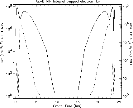at ISO altitudes comparable to that of GOES-9. Typical electron integral fluxes as a function of ISO orbital time are shown in Figure 5.5 for two energy cut-offs.

**Figure 5.5:** *Trapped electron fluxes as a function of ISO orbital time for two energy channels (100 keV and 4 MeV).*
$\resizebox {11cm}{!}{\includegraphics{NiemineP_2.eps}}$

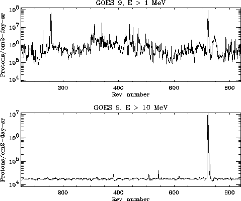
On the other hand, since the ISO mission was carried out nominally during the solar minimum period, the solar energetic particle contribution was not significant, except for two moderate solar proton events that took place towards the end of the mission: the first, a double-event in November 1997 (revolutions 720-722) during wich the proton flux for E

10 MeV and E

100 MeV increased by almost three orders of magnitude and almost one order of magnitude respectively with respect to its average value (see Figure 5.6); and the second, shorter one in April 1998, already during the so-called `Technology Test Phase' after helium boil-off^5.1. The first event was clearly registered by all four ISO instruments (a detailed description of the effects produced on the detectors is given in Heras 2001, [77]), while the second one had measurable effects on the ISO Star Tracker, as an increased false count rate. Neither of these events contributed significantly to the overall degradation of the satellite in comparison with the long term effect of the constant radiation belt traversals.

**Figure 5.6:** *Daily proton fluence measured by the GOES-9 satellite (Space Environment Center, NOAA) during the ISO mission.*
$\resizebox {11.5cm}{!}{\includegraphics{fig5_sp.ps}}$

During the science observation window the main source of radiation are galactic cosmic rays. They originate outside the solar system, and mainly consist of protons (85%), $\alpha$ -particles (14%), and a smaller component of heavier ions. The major part of these particles cannot be stopped by the spacecraft shielding since its differential spectrum peaks roughly between 500 MeV and a few Gev, and are therefore highly penetrating. Due to the high energies involved there is very little that can be done to exclude these effects, and increasing the shielding thickness may in fact be worse since more secondary particles (neutrons, protons, spallation products) can be generated, thus potentially adding to the problem (Nieminen 2001, [129]). The flux of cosmic rays is anticorrelated with the solar activity. This is because during the solar maximum period the expanding heliospheric magnetic field scatters more effectively the arriving charged particles. Apart from the slow variation over the solar cycle (not more than a factor of two in the integral proton fluxes) this radiation environment component is very stable.

5.6.1.2 Glitches in ISO detectors

The main effect produced in the detectors by the space radiation environment is the production of signal spikes or `glitches' caused by particle hits in the detectors. They can have negative or positive polarity and any amplitude between telemetry resolution and saturation.

The detector `background' resulting from the steady cosmic ray bombardment in the science windows, as well as by the energetic electron fluxes in the Earth's radiation belt and/or from their secondaries form the bulk of the glitches analysed by the four instrument teams.

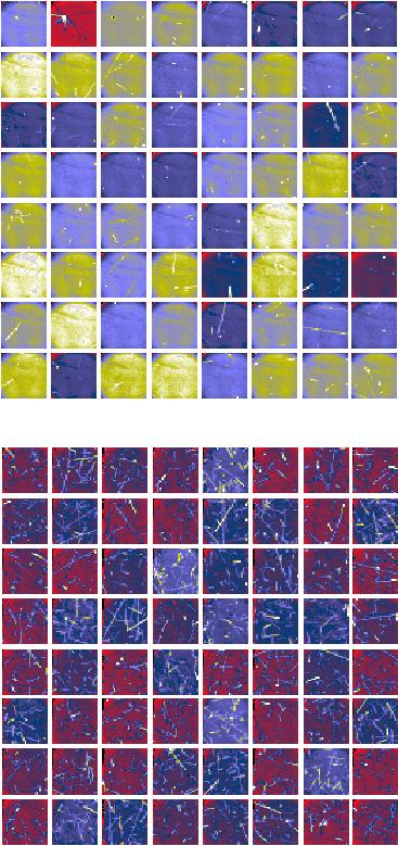
Upon impinging on the spacecraft, the incident particles can undergo various processes that lead to a modification of the radiation environment as seen at the instrument level. The highly energetic galactic cosmic rays and solar event protons that reach the detectors even after thick shielding leave a trace of ionisation along their track. This can be clearly observed as lines and spots in the detector pixel image, such as in the case of ISOCAM (see Figure 5.7, analysis done by Sauvage 1997, [143]). Numerous secondary particles such as $\delta$ -rays and neutrons can also be generated, leading to shower-type particle cascades.

**Figure 5.7:** *Sets of ISOCAM images taken during solar quiet period (upper panel) and during the solar proton event of 4-10 November 1997 (lower panel).*
$\resizebox {13cm}{!}{\includegraphics{NiemineP_5.eps}}$

With the minimum shielding of 9 mm Aluminum equivalent, electrons in the outer radiation belt need energies of at least $\sim$ 4 MeV to reach any of the ISO detectors. However, in slowing down in the shielding, the electrons generate bremsstrahlung photons that can be more penetrating that the incident electrons themselves. These electrons and photons may then be observed as an increase in the low-energy part of the glitch spectrum. The average energy deposited by a secondary electron, emitted on absorption of a bremsstrahlung photon is 0.1-0.2 MeV in Si and $\sim$ 0.1 MeV in Ge.

Table 5.2 displays the glitch rates per unit area for the different ISO detectors as measured in-orbit. The results show that when comparing values for the same detector material, the observed glitch rates agree within a factor of 2-3.

**Table 5.2:** *Comparison of observed glitch rates and minimum deposited energy in the ISO detectors.*
Detector type/	Glitch rate	Minimum deposited energy
Instrument	[cm $^{-2}$ s $^{-1}$ ]	[keV]
Si:Ga
CAM	14.9	-
PHT-P1	6.5	1
PHT-S	5.8	1
SWS	10.0	1
Ge:Be
LWS	6.3	1.9
SWS	17.8	0.95
SWS-FP	10.1	0.95
Ge:Ga
PHT-P3	10.1	1
PHT-C100	12.5	1
LWS	7.0	1.2
PHT-C200 (stressed)	7.3	1
LWS (stressed)	6.7	1.3

The same analysis can be made for the observed glitch height (deposited energy) distributions. Again, the results obtained are consistent for detectors made of the same material (Heras 2001, [77]).

Considering the diversity of instrument designs, instrumental data and software used, the differences found can be attributed to: i) instrument shielding; ii) cross-talk between detectors, iii) the efficiency in the detection of small glitches, which is particularly important because they are the most numerous; iv) the uncertainty in the values of the photoconductive gain (especially for LWS), which affects the conversion from voltage jumps to energy deposited in the detectors; and v) the number of undetected glitches due to saturation.

Glitch rates per unit area and glitch height (energy deposited) distributions can also be predicted for the different ISO instruments and detectors with the help of Monte-Carlo simulations based on ray-tracing techniques or with full simulations of the physical processes ocurring along the track of the incident particles and their secondary particles, taking into account also the local shielding (this second approach was only needed for LWS since for the other three instruments the ray-tracing method provided a fair agreement with in-flight data). A detailed description of the results obtained from these simulations can be found in Heras 2001, [77] and references therein.

The comparison of the observed energy deposited distributions with the results of ray-tracing simulations which model primary cosmic ray-induced glitches only shows a good agreement at high energies, but the peak of the observed distributions at the lowest deposited energies are not reproduced, especially in the Ge:Be detectors. In addition, the observed glitch rates are between 1.5 and 4 times higher than the predicted values. These facts, together with the correlation found between glitch rates and the electron flux measured by the GOES-9 spacecraft, lead to the conclusion that between 30 and 75% of the observed glitches are caused by $\delta$ -rays and other secondary particles produced by cosmic rays and the environment protons and electrons in the detectors and in the instrument and satellite shields (Heras et al. 2001, [78]).

Glitches were detected and removed from ISO data following deglitching algorithms implemented in the ISO Off-Line Processing pipeline. In some cases more sophisticated deglitching methods have been provided in the Interactive Analysis software packages. They are described in detail in Heras 2001, [77] and references therein, or in the instrument specific volumes (II to V) of this Handbook and, thus, will not be discussed here.

5.6.1.3 Other radiation induced effects on the detectors

Although radiation effects are mainly recognised by the presence of glitches in the science data, in some cases they are also associated with temporal changes in detector responsivity, dark current levels and noise.

SWS: The space radiation environment affected the long term behaviour of band 3 Si:As SWS detectors, causing their dark current levels, and in some cases, their dark current noise, to increase during the mission. The other SWS detector bands were stable and did not show long term trends. Some of the worse band 3 detectors cured spontaneously (e.g. detectors 34 and 36), that is, their dark currents and noise decreased suddenly to launch levels without apparent reason. Laboratory tests in which Si:As detectors were irradiated with 100 MeV protons during long periods reproduced successfully the in-orbit behaviour. Although no curing procedure could be found, it was decided to operate the detector at a lower bias than initially planned, which reduced the damaging radiation effects and kept the dark currents and noise at acceptable levels during the mission (Heras et al. 2001, [78]).

LWS: A similar behaviour was observed in LWS detectors. Sudden voltage jumps produced by impacts affecting a given integration ramp were followed by a change in the detector responsivity in the following ramps. In addition to these `positive' glitches, `negative' ones have also been found. These caused a sudden decrease in the ramp voltage, and are thought to be produced by hits on the FET. Negative glitches did not appear to affect the detector responsivity (Swinyard et al. 2000, [156]). The overall responsivity of the detectors increased with particle hits during the orbit. To re-normalise the responsivity, the bias current was increased beyond the breakdown voltage for each detector twice in every orbit: a first bias boost on exit from the Van Allen belts; and a second one half way through the 24 hour orbit. Dark currents were not affected by the cosmic rays and remained constant during an orbit. The change in responsivity between bias boosts was monitored by the use of the infrared illuminators. This way it was possible to correct for the overall drift in responsivity with time during an orbit in the processing pipeline.

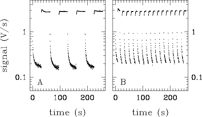
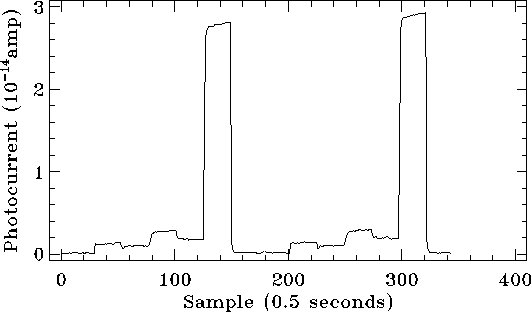
CAM: In ISOCAM, responsivity variations were also detected after perigee passage due to the very high radiation dose coming from trapped particles in the Van Allen belts. In extensive radiation tests performed before launch it was already found that $\gamma$ -ray sources, protons and heavy ions impacting the detectors induced a responsivity increase which relaxed in a few hours. The effect was minimised if the photo-conductor was polarised and exposed to a high infrared flux. In-orbit, during the perigee passage, since the instrument was switched-off, a specific power supply kept a bias voltage on the photo-conductors, and the camera was left open to light. The responsivity variation often remained below 5% in the science window. Appart from common glitches, other types of glitches were detected in ISOCAM data and classified as: faders, where the pixel value decreases slowly until a stabilised value is reached (Figure 5.8); and dippers, where the pixel value decreases first below the stabilised value, and then increases slowly until the stabilised value is reached (see Figure 5.9). While common glitches are interpreted as induced by both trapped and galactic protons and electrons, faders would be induced by energetic protons, electrons and light galactic ions, and dippers would be induced by heavy galactic ions (Claret et al. 2000, [25]). The effect of glitches are not so dramatic for SW detectors as for LW detectors. This is because the active zone of the pixel is very thin,

10 $\mu$ m, so that its volume is very small. Due to the very low energy needed to create a free carrier pair, the charge generation is equivalent for both SW and LW detectors, but the pixel geometry of the SW array ensures that most of the particles cross only one pixel. After a hit the responsivity of the pixel decays slowly to its previous value. The decay time is the same as for transients due to IR flux changes (see Section 5.6.2). The lower the illumination of the array, the longer the decay time.

**Figure 5.8:** *Temporal flux history of a pixel of the LW detector array which was hit by a* *fader* *glitch, showing a long tail. The flux in ADU is plotted against time given by the exposure index. The large structure corresponds to a source detection.*
$\resizebox {12cm}{5cm}{\includegraphics*[90,375][550,710]{fig_glitch_h1.ps}}$

**Figure 5.9:** *Temporal flux history of a pixel of the LW detector array which was hit by a* *dipper* glitch with a negative tail. The flux in ADU is plotted against time given by the exposure index. Note the gain variation of about 5 ADUs which appears after the second glitch.
$\resizebox {12cm}{6cm}{\includegraphics*[90,555][555,710]{dipper.ps}}$

PHT: The continuous hits of high energy particles during the ISO orbit also increased the responsivity of PHT detectors at short term and long term scales. At short term scales the disturbance of an integration ramp after a hit was usually followed by a tail-like signal excess lasting a few integration ramps, which is interpreted as a momentary response variation. At long term scales, already during the pre-flight calibration tests it was found that the responsivity of the detectors increased after exposing them to high energy radiation. The same behaviour was found in-orbit, affecting mostly the responsivity of the Ge-based, low bias voltage far-infrared detectors (P3, C100 and C200), whereas the Si-based, high bias voltage detectors P1, P2 and PHT-SS showed only small changes in their responsivity. An exception was the PHT-SL array which showed a similar, but less pronounced behaviour as the FIR detectors. This change of responsivity was also found to be correlated in-orbit with the geomagnetic activity and the electron fluxes, increasing systematically (by 20-50%) one or two days after the onset of a geomagnetic storm. P3 and C100 showed the largest changes, followed by C200 (Castañeda & Klaas 2000, [14]). Due to the high radiation doses during perigee passage the responsivities and noise levels of the ISOPHOT detectors were strongly increased before the beginning of every new science window. Therefore, appropriate curing procedures were designed for the different detectors to restore the nominal responsivities. The procedures were applied after the switch-on of the instrument, before the beginning of the science window. For the doped germanium detectors (P3, C100 and C200) they consisted of a combination of bright IR-flashes using one of the FCSs and a bias boost (absolute increase of the bias voltage). For the doped silicon detectors (PHT-SS, PHT-SL, P1 and P2) curing was achieved by exposing the detector to a higher temperature at a reduced bias voltage for a defined period of time. In addition, P1 underwent an infrared flash curing. The doped germanium detectors were much more susceptible to drifts caused by accumulating effects of the high energy radiation impacts. In order to keep their responsivities within the nominal range a second curing procedure was applied around apogee passage in the handover window, when the satellite control was switched from VILSPA (Madrid) to Goldstone (California). Trend analysis performed immediately after the curing procedure showed that the nominal responsivities were re-established with $\pm$ 2% accuracy for all detectors, if the space environment conditions were stable. On the other hand, low energy glitches also affected the measurements by increasing the dark current level and the detector noise. The consequence was an increase of the minimum measurable signal, or equivalently, a decrease of the sensitivity limit. All these effects are associated with the generation of electron-hole pairs in the bulk of the detectors during the irradiation, and with the capture of the minority carriers by the compensating impurities.

5.6.2 Detector transients

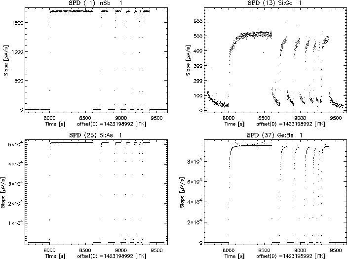
The operation of infrared detectors in space is strongly complicated by memory effects. These detectors are usually doped silicon and germanium bulks with implanted low ohmic contacts used as extrinsic photoconductors and are characterised by a transient response after flux changes.

A large number of such detectors were used on board ISO (see Table 5.3). From this point of view, the ISO satellite was a very interesting laboratory since several technologies and detector materials (Ge:Be, Ge:Ga, In:Sb, CID In:Sb, Si:As, Si:Ga, Si:B) were used to cover a wide spectral range from 2.5 to 240 $\mu$ m.

**Table 5.3:** *List of the IR detectors on board ISO with indications of type, operating wavelengths (peak or range) and detector topology (individual pixel, linear or matrix array).*
	Detector Name	Type	Wavelength ( $\mu$ m)	Pixels
CAM	SW	CID In:Sb	2.5 - 5.5	$32\times32$
	LW	Si:Ga	4.0 - 18.0	$32\times32$
PHT	SS & SL	Si:Ga	15, (peak)	64 $\times$ 1
	P1	Si:Ga	15, (peak)	1
	P2	Si:B	25, (peak)	1
	P3	Ge:Ga	100, (peak)
	C 100	Ge:Ga	100, (peak)	$3\times3$
	C 200	Ge:Ga (stressed)	180, (peak)	$2\times2$
SWS	band 1	In:Sb	2.38 - 4.08	$1\times 12$
	band 2	Si:Ga	4.08 - 12.0	$1\times 12$
	band 3	Si:As	12.0 - 29.0	$1\times 12$
	band 4	Ge:Be	29.0 - 45.2	$1\times 12$
	FP band 5	Si:Sb	11.4 - 26.	$1\times 2$
	FP band 6	Ge:Be	26.0 - 44.5	$1\times 2$
LWS	SW1	Ge:Be	43 - 51	1 detector
	SW2-SW5, LW1	Ge:Ga	50 to 121 (10)	5 detectors
	LW2-LW5	Ge:Ga (stressed)	108 to 197 (20)	4 detectors

Some of these detectors exhibit long time constants and it was usually not possible to wait for current stabilisation when they were exposed in space to sources of infrared emission, making the determination of the input fluxes a very difficult task. Without any correction, the errors induced by the transient effects can be as large as 50% in some cases. However, in some of the ISO detectors and under certain circumstances, the response after a flux change was highly reproducible, which gives sense to look for models and to correct the data for these transient effects.

Before launch, ground-based tests were extensively performed (CAM - Pérault et al. 1994, [136]; PHT - Groezinger et al. 1992, [65]; Schubert et al. 1994, [146]; Schubert 1995, [145]; SWS - Wensink et al. 1992, [164]). Unfortunately, as a result of these ground-based tests it was not possible to develope and accurate model for transients in SWS and CAM. Only for PHT-S a promising non-linear model was proposed (Fouks & Schubert 1995, [54]), that was later corrected to introduce the effect of temperature variations.

During the ISO mission, several linear and non-linear models were suggested for the various ISO instruments and observing modes. It became evident that the models should be non-linear and non-symmetrical and take into account the illumination history of the detector.

Analytical models were developed for infrared detectors by Vinokurov & Fouks 1991, [162], from the non-linear equations describing such detectors (Vinokurov & Fouks 1991, [162]; Haegel et al. 1999, [71]). One of these models, the so-called `Fouks-Schubert' model (Fouks & Schubert 1995, [54]), was the one used for describing transients in PHT-S detectors during the ground-based tests, as we have already mentioned. This is a simplified analytical model which is able to reproduce the behaviour of Si:Ga detectors which high accuracy.

The Fouks-Schubert model and the basic equations involved are described in Coulais et al. 2000, [36], and references therein. The Fouks-Schubert formula, which describes the detector behaviour when starting from an unstabilised current $J_{n-1}^{end}$ at the end of block

is:

where the time

is measured from an arbitrary instant after the flux change at time

, $\beta$ is the instantaneous jump and $\lambda$ is a constant. The unstabilised current $J_{n-1}^{end}$ before the flux change reflects the history of the detector (stabilisation in block

is achieved when $J_{n-1}^{end} = J_{n-1}^{\infty }$ ); $J_{n}^{\infty }$ is the steady-state current under the constant incoming flux during block

This simple non-linear analytical formula (Equation 5.2), which takes into account the memory effects, describe the processes in the detector bulk, with the use of Fouks' boundary condition (Fouks 1981a, [50]; 1981b, [51]) that describes the properties of the detector contacts. This boundary condition has the form:

where $p\left( {z,t} \right)$ is the hole concentration at the plane

measured from the injecting contact placed at the plane

, the time

is measured from an arbitrary instant, as in Equation 5.2, $\Delta E\left( {0,t} \right)$ is the change of the near-contact field with time ( $\Delta E ( {0,t} ) = E( {0,t} ) - E( {0,0})$ ), and $E_{j}$ is the injection ability of the contact. Equation 5.3 allows to describe the contact properties with a high precision (Fouks & Schubert 1995, [54]) and, in addition, to take into consideration additional technological and engineering effects inherent to real detectors (Fouks 1997, [52]).

The use of Equation 5.3, instead of a detailed consideration of the processes which occur inside the near-contact space-charge region, strongly simplifies the description of transient currents. Nevertheless, in general the problem remains rather complex even after this simplification. However, in the case where $E_{j}$ is much less than the steady-state field in the detector bulk $E_{0} = V_{0}/l$ (where $V_{0}$ is the steady-state voltage applied to the detector,

is the inter-contact distance), this description can be additionally strongly simplified, and Equation 5.2 serves as a very exact description for transient currents (Vinokurov & Fouks 1991, [162]). The parameter $E_{j}$ quantifies the quality of the contacts and depends on the flatness of the donor profile in the near-contact region and is linked to the time constant of the current relaxation. The higher the contact quality, the less is $E_{j}$ , and the shorter the time constant. In real detectors at liquid helium temperatures $E_{j}$ is of the order of 10 $^{2}$ -10 $^{3}$ V/m. For Si:Ga detectors $E_{0}$ is considerably high, typically 10 $^{5}$ -10 $^{6}$ V/m, which provides a very high accuracy to Equation 5.2. In Ge:Ga detectors $E_{0}$ , however, $E_{0}$ is of the order of $E_{j}$ , thus making this formula not so exact.

The other important point lies in the fact that Equation 5.2 is applicable only when the illumination is uniform on the pixel surface. In this case, high photoelectric non-stationary cross-talking between adjacent pixels, that are inherent to such detectors (Fouks & Schubert 1995, [54]), compensate each other, which makes the electric field uniform along the planes

and the used one-dimensional equations true. Under non-uniform illumination the set of one-dimensional equations cannot be used, and Equation 5.2 looses its accuracy (Vinokurov & Fouks 1988, [161]; Vinokurov et al. 1992, [163]).

5.6.2.1 Si:Ga detectors

Several Si:Ga detectors were on board ISO (see Table 5.3): the LW 32 $\times$ 32 matrix array of ISOCAM; the band 2 (a 1 $\times$ 12 linear array) of SWS; and the PHT-SS, PHT-SL and P1 detectors of ISOPHOT.

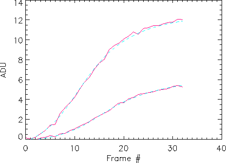
The LW detectors of ISOCAM present strong transient effects. The worst situations occurred in two cases:

The transient behaviour of the LW channel has two main components (see Figure 5.10): a short term one which consists of an initial jump typically of about 40-60% of total signal step, followed by a long term drift with small amplitude oscillations (typically 5-10 $\%$ of the flux) and can last hours (Abergel et al. 2000, [1]; Coulais & Abergel 2000, [35]).

**Figure 5.10:** An example of the transient behaviour of LW-CAM detectors. This is an observation which starts just after the switch-on of the instrument at the begin of a revolution. We clearly see the two components of the transient response: the short term transient from time $\sim$ 0 s to $\sim$ 50 s, which is the transient response described by the Fouks-Schubert model and, from $\sim$ 100 s to the end, the response change due to the long term drift.
$\resizebox {11cm}{!}{ \includegraphics*[5,5][480,330]{fig1_transient_long.eps}}$

Upward and downward steps are not symmetrical (downward steps are hyperbolic-like) and the short term response at a given time strongly depends on the past of the observation and also on the spatial structure of the input sky (e.g. uniform emission or point sources).

Under quasi-uniform illumination the short term transient response of individual LW pixels can be described by the Fouks-Schubert model with an accuracy around 1 $\%$ per readout for all pixels except near the edges. (Coulais & Abergel 2000, [35]). This model is fully characterised by the two parameters ( $\beta$ , $\lambda$ ) above mentioned, which are determined for each pixel in the array. No significant changes of these parameters were observed during the whole in-orbit ISO life per pixel, so that only one 32 $\times$ 32 map for each parameter was used when this correction was applied in the data reduction pipeline. In addition, the dispersion found in the values derived from pixel to pixel indicates that:

In the LW array, the pixels are defined only by the electrical field applied between the upper electrode and the bottom 32 $\times$ 32 contacts. As a consequence of the electrical design of the matrix array, the adjacent pixels are always affected by cross-talk effects (Vigroux et al. 1993, [160]). Under uniform illumination these cross-talks compensate each other and can be ignored but this is not the case when the input sky contains strong fluctuations with typical angular scale around the pixel size (e.g. point sources with gradient between pixels typically higher than 20 ADU/s). Thus, the one-dimensional Fouks-Schubert model fails for such point sources, and three-dimensional models are required.

The LW-CAM data contained in the ISO Data Archive are corrected for transients using the `standard' one-dimensional Fouks-Schubert model above described. This means that the results obtained in fields with bright point sources or very steep gradients after applying this correction are not so accurate, although this is still within the few percent level.

Recently, a new simplified three-dimensional model for point source transients has been developed by Fouks & Coulais 2002, [53]. This model uses the same ( $\beta$ , $\lambda$ ) parameters which were used for the uniform illumination case and is able to qualitatively reproduce real point source transients. The model predicts e.g. that, starting from the same initial level, the stronger the source the faster the transient response and the higher the initial overshoot, as it is observed in real data, and it works better for configurations in which the PSF is narrow. A more complicated three-dimensional model, able to account for quantitative effects taking into account the true geometrical and electrical specifities of LW detectors, is still under development

With respect to the remaining effects above mentioned (long term drift, small amplitude oscillations,..) no physical models exist yet to describe the detector behaviour and only empirical dedicated processing methods have been developed so far. Two approaches exist for the extraction of reliable information from raster observations affected by long term drifts. For the case of faint point sources, as in cosmological surveys, source extraction methods are discussed in Starck et al. 1999, [152] and Désert et al. 1999, [45]. For raster maps with low contrast large-scale structure (as in the case of diffuse interstellar clouds) a long term drift correction method is available in CIA. This method was developed by Miville-Deschênes et al. 1999, [121] and is based on the use of the spatial redundancy in raster observations to estimate and to correct for the long term drift (see Figure 5.11).

**Figure 5.11:** When the contrast of the observed object is very low, and when the observations suffer from long term transient effects, it is important to use a correction method based on the spatial redundancy in raster observations. In the present case, the structure of a low contrast diffuse interstellar cloud is recovered (see Miville-Deschênes et al. 1999, [121] for more details).
$\resizebox {15cm}{!}{\includegraphics{ESA_info_note.ps}}$

For ISOPHOT Si:Ga detectors (P1, PHT-SS and PHT-SL detectors), and although a good agreement was achieved between transients and Fouks models during ground-based tests, the application of these models to real in-flight data was unsuccessful. Several facts can explain the change in the behaviour of the detectors:

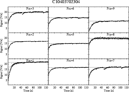
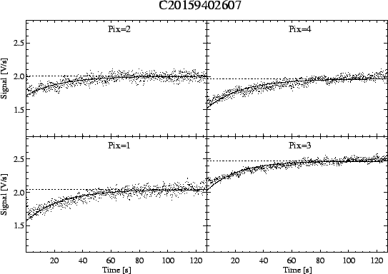
Typical drift curves in P1 detectors are shown in Figure 5.12. In case of a flux drop, a signal decay and in case of increasing flux steps, a signal rise is observed. In addition, a hook response during the first 40 seconds is also observed for large positive flux steps. The signal shows a behaviour similar to a strongly damped oscillation around the asymptotic level. For even higher flux steps the signal behaviour can be restricted to an overshoot followed by a slow decay. Doped silicon detectors tend to show a longer stabilisation time than doped germanium detectors (P3, C100 and C200 in the case of ISOPHOT), which can go from just a few seconds to hours. The relative stabilisation time is faster for positive flux steps. and steps at low flux levels take more time to stabilise. In addition, the stabilisation time also depends on the temperature of the detector.

**Figure 5.12:** Examples of P1 detector transients. Left panel (A): 4 transient curves after a flux step overplotted in the same graph for comparison, the highest curve corresponds to the largest positive flux step. In all cases the signal prior to each step was the same and had a strength of about 35 V/s. For these flux steps a signal overshoot is detected followed by a strongly damped oscillation. Right panel (B): multi-filter observation of the star HR6705, filter sequence P_16 (64 s integration), P_3.6 (64 s) followed by the P_3.6 (32 s) FCS measurement. Both the P_16 as well as the P_3.6 FCS measurement show a downward drift, with a longer stabilisation time for the fainter P_16 signal.
$\resizebox {14cm}{!}{\includegraphics{driftfig1.eps}}$

In OLP no sophisticated treatment of transients was applied to staring PHT-P1 observations. Instead, an algorithm was used which determines per chopper plateau whether a significant signal drift is present based on the application of the non-parametric Mann statistical test to the signals (Hartung 1991, [74]). In case such a drift is found, only the last stable part of the chopper plateau is used. Of course, this correction only works satisfactorily for measurements which are long compared to the stabilisation time. This `drift recognition' method is explained more in detail in Section 7.3 of the ISO Handbook Volume IV on ISOPHOT, [107].

In the case of chopped PHT-P1 observations, non-stabilised signals cause significant losses on the true difference signal. Signal derivation in OLP relies on the analysis of signals from pairs of consecutive readouts rather than signals per ramp. This gives better statistics of the signals per chopper plateau, since in many chopped measurements each chopper plateau covers only a few (typically 4) ramps. To increase further the robustness in determining the difference signal, the repeated pattern of off-source and on-source chopper plateaux is converted into a `generic pattern'. The generic pattern consists of only 1 off- and 1 on-source plateau and is generated using an outlier resistant averaging of all plateaux. The shape of the generic pattern determines the correction factors to apply with regard to stabilised staring measurements of a sample of calibration standards.

For PHT-S observations taken in staring mode an alternative approach was developed, known as the `dynamic calibration' method, which performs the calibration measurement by comparing the transient behaviour of the unknown source with that of celestial standards of similar brightness. Then, the transients which show the same time scale and amplitude for both measurements cancel out in the calibration process. This method works only for staring PHT-S observations because the flux history of PHT-S pixels is similar in all observations as they always start with a 32 s dark measurement which is followed by the real measurement. A detailed description of how the flux assignment is performed and the library of calibration standards and model spectra used for the application of this method can be found in García-Lario et al. 2001, [60]. The `dynamic calibration' brings down the errors associated to this observing mode (sometimes as high as 30%) to just a few percent.

Note that this accuracy is not applicable to raster measurements made with PHT-S, which also generally suffer from transient effects, because the assumption of a flux history similar to that used for the calibration stars is not met for all raster points in a map except for the first one. Thus, only a static spectral response function can be applied in this case. The photometric calibration of each raster point is performed by converting the signal to a flux using an average spectral response function for PHT-S staring observations derived from 40 observations of 4 different standard stars with different brightness.

The same argument is applicable to chopped PHT-S observations. Thus, for this observing mode a `drift recognition' routine similar to the one used for P1 detectors was implemented in OLP to detect the presence of a significant signal transient on a chopper plateau. When a transient is detected, a range of unreliable signals are flagged. The signal so derived is then corrected assuming a spectral response function corrected for chopper losses. The Fouks-Schubert model is not applicable in this case because the sources are usually very faint and the signal-to-noise ratio is too low for the fitting procedure to work properly. Thus, although the possibility exists in PIA of applying the Fouks-Schubert correction to faint sources observed in chopped mode, the above alternative approach was used to calibrate these sources in the automated pipeline. More details on the method applied and the calibration of the standard stars used for this purpose are given in García-Lario et al. 2001, [60].

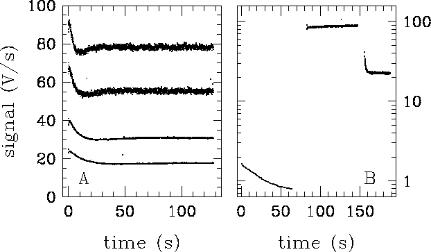
An overview of the various transient behaviours observed for the different SWS bands as a function of the detector material is shown in Figure 5.13, where we can see that band 2 (Si:Ga) and band 4 (Ge:Be) are those affected by the largest memory effects.

**Figure 5.13:** *Example of the various transient behaviours observed for the different SWS bands as a function of the detector material (Band 1: InSb; Band 2: Si:Ga; Band 3: Si:As; Band 4: Ge:Be).*
$\rotatebox {90}{\resizebox{13.5cm}{!}{\includegraphics{from_do.ps}}}$

The signature of memory effects in the Si:Ga band 2 of SWS is that the up- and down-scans are different in flux level (up to 20% for sources with fluxes greater than about 100 Jy). The down-scan normally succeeds the up-scan in the AOT and appears to be already `accustomed' to the flux level.

For band 2 SWS data, an adapted version of the Fouks-Schubert model was developed by Do Kester (Kester 2001, [98]) and successfully implemented in the legacy version of the SWS pipeline to correct this band for transient effects as well as in the Observers' SWS Interactive Analysis (OSIA) software package (version 3.0). The method brings the errors (sometimes up to 20% originally) down to the few percent level.

A complete description of the procedure followed and how the correction was implemented in the pipeline can be found in the ISO Handbook Volume V on SWS, [108]. Additional details are provided in Kester 2001, [98] and García-Lario et al. 2001, [60].

5.6.2.2 Ge:Ga detectors

Several Ge:Ga detectors were also set up for use on board ISO (see Table 5.3): one detector (P3) and two small matrix arrays for PHT (C100 3 $\times$ 3 pixels and stressed C200 2 $\times$ 2 pixels); and several stressed (4) and un-stressed (5) monolithic detectors for LWS. All of these detectors were affected by transient effects which can bias the final photometry typically from 10 to 40%.

As we have already mentioned, the present status of our understanding of transients in Ge:Ga detectors is less favorable than for Si:Ga detectors. Based on the ratio $E_{0}/ E_{j}$ , Ge:Ga detectors are unfortunately always in an unfavourable domain for the application of the Fouks-Schubert model correction.

At first sight these transients appear easier to model than the Si:Ga ones because they are at first order exponential (Church et al. 1993, [22]). Thus, the use of non-linear models seems to be a priori less necessary in order to take into account the memory effects. However, the correction is not as precise as the one obtained for Si:Ga detectors using non-linear models. The expected accuracy of such simplified analytical models, even if the detector is perfect, is only about 10-20 $\%$ . The main problem is that some very important characteristics of such detectors are often not well under control (e.g. contact quality). and, thus, each Ge:Ga detector seems to require a peculiar model (Coulais et al. 2000, [36]).

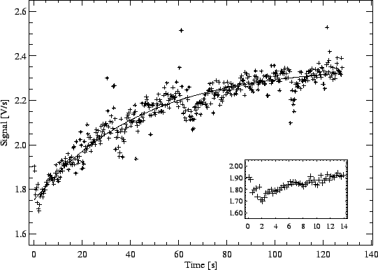
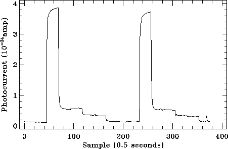
In general, doped germanium detectors show faster stabilisation times than doped silicon ones (typical time scales are 100 s for P3 and C100, 40 s for C200, and 50 to 100 s for LWS detectors). Some of them present an initial hook response (quick overshoot) for high upward steps of flux and undershooting after a downward step. The long term response exhibits a time constant which decreases for high fluxes, whereas it strongly increases for low fluxes. This transient component can be well modelled by an exponential function in most cases (Acosta-Pulido et al. 2000, [8]).

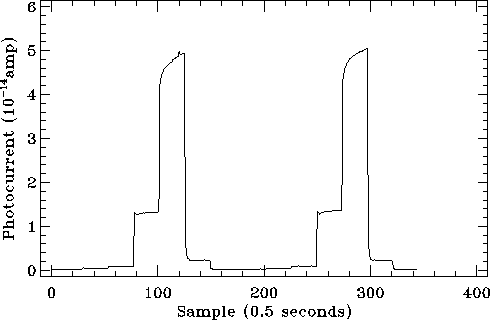
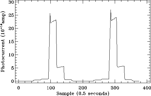
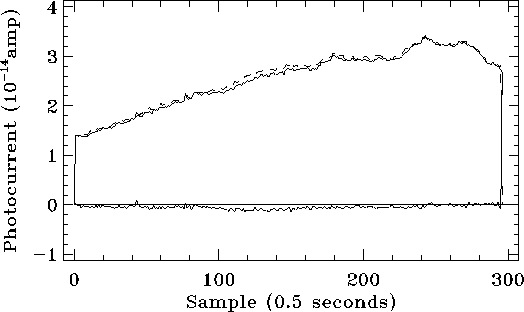
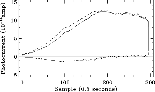
Figures 5.14 and 5.15 show the typical transient behaviour observed in P3 detectors at intermediate and low flux levels, respectively. We can see the initial hook response clearly in the intermediate flux example and the longer stabilisation time for low fluxes. In both cases the long term transient behaviour has been modelled with a single exponential function which can be written as:

**Figure 5.14:** Typical transient behaviour of detector P3 at intermediate flux level ( $\sim$ 11 Jy at 100 $\mu$ m). The measured signals are represented by plus sign symbols. Detected glitches are marked by crosses. The single exponential model is represented by the continuous line through the data points. The initial signal sequence is shown in the inset, where the hook response is clearly recognised.
$\resizebox {12cm}{!}{\includegraphics{P30644800704.eps}}$

**Figure 5.15:** *Typical transient behaviour of detector P3 at low flux level ( $\sim$ 2 Jy at 100 $\mu$ m). The meaning of the symbols is as in Figure 5.14.*
$\resizebox {12cm}{!}{\includegraphics{P30073401910.eps}}$

The first analysis shows that $\tau$ is inversely proportional to the final signal, $S_{\infty}$ , in log-log scale (see Acosta-Pulido et al. 2000, [8]). Therefore, $\tau$ can be written as an inverse power law function of $S_{\infty}$ . The parameter $\alpha$ describes the behaviour of the transient effects with the illumination and

is a normalisation constant.

and $\alpha$ are parameters which have to be determined for each detector/pixel. In the case of the Fouks-Schubert function $\alpha$ is equal to unity. If the proposed function is a good description of the transient behaviour of the considered detectors, those parameters can be fixed. The stabilised signal is obtained by fitting the above function to the measured signals and leaving $S_{ini}$ and $S_{\infty}$ as free fit parameters.

The parameters

and $\alpha$ for the detectors P3, C100 and C200 were determined in-orbit using a large set of long measurements. The measurements were selected if a clear transient behaviour was present, and they were long enough that at the end the photocurrent is close to stabilisation. Nevertheless, this data set may suffer some selection bias: transients with very long time constants (

1000 s) could not be detected because of the limited observing time; and the flux history may influence the transient as well as the switch-on of the detector every time an observation starts. In the process of determining

and $\alpha$ each measurement was fitted by leaving all parameters free in the above expression and rejecting those fits where the residual rms per degree of freedom was larger than 3.

**Table 5.4:** *Time constants for the long term transients observed in P3, C100 and C200 detectors derived from the empirical model*
Detector		$\alpha$		$\beta$
P3	87 $\pm$ 8	0.79 $\pm$ 0.05	0.79	$\sim$ 0.34
C100	36 $\pm$ 3	0.48 $\pm$ 0.04	0.63	$\sim$ 0.30
C200	38 $\pm$ 2	0.63 $\pm$ 0.03	0.89	$\sim$ 0.85

The results obtained from a least square fit are presented in Table 5.4, together with the correlation coefficient

. For P3 and C200 the correlation is very good while it is worse for C100.

We perfomed tests using an independent set of measurements other than those used for determining the time constants. The resulting ${\chi}^2$ distributions are very narrow and peak around 1. The worst case is again the detector C100, for which the ${\chi}^2$ distribution for all pixels (except pixel 8) is wide and values around 2-3 are frequent. The low frequency noise which affects detectors C100 and P3 when measuring faint targets is likely limiting the goodness of the fit.

According to the values derived and shown in Table 5.4 it is also possible to estimate the fraction of the final signal which is affected by the slow transient component, i.e. the signal difference between the value reached at the initial jump and the final value. The magnitude of this component combined with the time constant determines the accuracy of any measurement after a certain time. For example, a long time constant is not so relevant, if the fraction of the slow component is small compared to the total signal. The magnitude of the slow component can be estimated from the initial jump after a flux change and the knowledge of the final stable current. This has to be derived from chopped measurements where the flux changes are like a step-function. Raster observations cannot be used, because the flux varies gradually as the telescope slews to a different sky position. Results for detectors P3, C100 and C200 are presented in Table 5.4, where $\beta$ represents the fraction of the total signal difference which is achieved immediately after the flux change. It has been found theoretically that the magnitude of the slow component increases with the photoconductive gain,

(Haegel et al. 1996, [70]).

depends on the material, the electric field and the dimensions of the detector. Detectors P3 and C100 are manufactured of the same material but they have different bias voltages and dimensions, yielding

; which is consistent with a larger fraction of the slow component for C100.

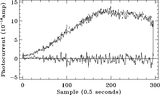
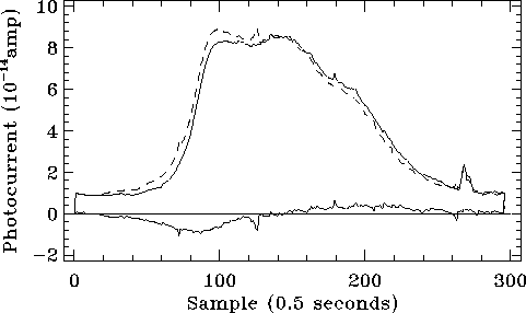
We present in Figure 5.16 an example of the application of this single exponential fit model to a measurement taken with detector C100: using the full measurement time of 512 s an error of 6% between the direct measurement of the signal and the model prediction is found. A comparison of the estimates of the final signal using only the first 32 s gives the following results: the value obtained from the `drift recognition' method which is applied in the pipeline is too low by 30%, whereas the value obtained from the empirical model above described is lower by only 12%. This example demonstrates how the use of this method can significantly improve the photometric accuracy of relatively short measurements.

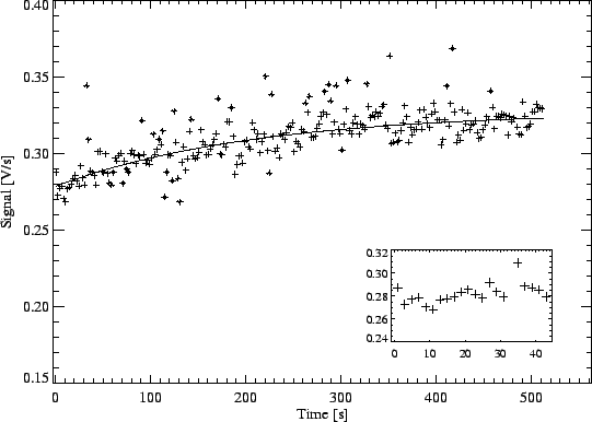
**Figure 5.16:** Typical transient behaviour of the nine C100 pixels at high flux level ( $\sim$ 75 Jy at 80 $\mu$ m). The dots represent the measured signals, the solid line the fit and the dashed horizontal line the predicted final signal level.
$\resizebox {12cm}{!}{\includegraphics{C10403702304.eps}}$

Another example, this time applied to detector C200, is shown in Figure 5.17. Again, a single exponential fit has been applied to predict the final signal level with a quite satisfactory result.

**Figure 5.17:** *Typical transient behaviour of the four C200 pixels at high flux level ( $\sim$ 60 Jy at 150 $\mu$ m). The meaning of the symbols is as in Figure 5.16.*
$\resizebox {12cm}{!}{\includegraphics{C20159402607.eps}}$

However, a detailed analysis of the transient curves, especially for detector C100, reveals the presence of more than one time constant. Solutions consisting on a combination of two (and even three) exponential functions have been found to describe better the drifting curve improving the accuracy of the photometry (Church et al. 1996, [23]; Fujiwara et al. 1995, [56]). Currently, several fitting methods are available in the PIA software used for interactive analysis (Gabriel & Acosta-Pulido 1999, [57]). The main difficulty is to determine the relative importance of the different components.

In the pipeline, a simple `drift recognition' method similar to the one applied in Si:Ga detectors is implemented for PHT-P3 and PHT-C staring observations. If the stability test fails for a given measurement, a empirical solution based on the fitting of an exponential function is tried (Schulz et al. 2002, [148]). Thus, as for the PHT-P1 detectors, the transient correction applied only works satisfactorily for measurements which are long compared to the detector stabilisation time at a given illumination.

In the case of chopped measurements, where non-stabilised signal causes significant losses to the true difference signal, OLP makes use of a `pattern recognition' method similar to the one used also for PHT-P1 detectors. For P3 detectors the accuracy is poor when the fluxes are below between 0.2 and 1 Jy (the exact number depends on aperture size and chopper throw), due to cirrus confusion and the restricted number of sky references longward of 80 $\mu$ m. For C100 and C200 the accuracy is also strongly limited when the fluxes detected are below 0.2 Jy and 1 Jy, respectively. In this case the chopper offset correction, being the zero point of the signal correction, is less accurate and the relatively bright sky background and the small number of reference positions make an estimation of the cirrus confusion noise necessary.

Finally, no transient correction was implemented in the pipeline for PHT32 chopped raster maps because of the high interactivity needed in the processing to correct these maps for transient effects. A processing tool including full transient modelling developed by Richard Tuffs (from MPI-Heidelberg) is available in PIA and details on its application to real data can be found in the proceedings of the ISOPHOT Workshop on P32 Oversampled Mapping, [149].

LWS Ge:Ga detectors present also memory effects, due to their slow response times (typically tens of seconds, as already mentioned) to changes of illumination (Church et al. 1992, [21]). As for the other Ge:Ga detectors on board ISO the typical transient behaviour of both LWS stressed and unstressed detectors consists of a long term component due to the steady accumulation of particle hits during each revolution and a short term component caused by the changes in flux.

In general, after a flux change, the immediate reaction is quick, and in some cases the detector overshoots, producing the characteristic hook response, but the detector output can take a considerable time to settle the final level. Specific laboratory tests were made before launch (Church et al. 1996, [23]) showing that the detectors actually react on a variety of time scales depending on the initial and final flux levels.

Church et al. 1996, [23] found that the response of LWS Ge:Ga detectors to a step change in flux could be modelled empirically by a function containing three exponential time constants, with typical values of

1, 5 and 30 seconds (for unstressed Ge:Ga detectors) and 0, 10 and 100 seconds (for stressed Ge:Ga detectors). However, the general behaviour and appearance of the hook response depends on bias and operating temperature, as well as on the flux levels. The main difference between the stressed and unstressed Ge:Ga detectors is in the speed of the hook response (faster in the stressed Ge:Ga detectors). The time constants generally decrease with increasing flux step. In all cases the transient response after a decreasing flux step is faster than the response after an increasing flux step. Kaneda et al. 2001, [92] uses a step and two-component exponential model to fit the step response of these detectors and shows that the transient response time decreases with an increase in both the initial and final incident flux levels.

The in-orbit transient response of the detectors is most clearly seen in the illuminator flashes that provide the basic sensitivity drift calibration. These are steps in flux levels that mirror the laboratory tests, but these sequences are much shorter and not all the effects appear as described above. Sample illuminator flashes are shown in Figures 5.18 and 5.19 for detectors SW4 (unstressed Ge:Ga) and LW2 (stressed Ge:Ga) respectively, which are those affected by the largest transient effects. For these detectors the slow long term response is the main problem as the flux is still increasing at the end of the flash. SW3 (unstressed Ge:Ga) and LW4 (stressed Ge:Ga) also show the same effect to a lesser extent. The remaining detectors are rather better behaved, e.g. the stressed LW5 (see Figure 5.20), although LW1 (unstressed) and LW3 (stressed) invariably show also a hook response.

**Figure 5.18:** *Typical transient behaviour observed in LWS-SW4 (unstressed Ge:Ga) detector under a series of illuminator flashes. This is one of the LWS detectors showing the largest memory effects.*
$\resizebox {12.4cm}{!}{\includegraphics{lloydc3_2.eps}}$

**Figure 5.19:** Typical transient behaviour observed in LWS-LW2 (stressed Ge:Ga) detector under a series of illuminator flashes showing an initial hook response and then a slow continuous rise typical of a long time constant.
$\resizebox {12.4cm}{!}{\includegraphics{lloydc3_3.eps}}$

The effect of the detector transient response on the illuminator flashes is to introduce a non-linearity into the drift correction. The problem is not that the correct illuminator flash level is not reached, but that the detector will respond differently depending on the flux levels involved, so the calibration will be inconsistent. How inconsistent will depend on the change in flux levels and the severity of the detector transient response.

**Figure 5.20:** *Typical transient behaviour observed in LWS-LW5 (stressed Ge:Ga) detector under a series of illuminator flashes. This is one of the better behaved LWS detectors.*
$\resizebox {12.4cm}{!}{\includegraphics{lloydc3_4.eps}}$

One of the major effects of this transient behaviour is in the determination and application of the so-called `Relative Spectral Response Function' (RSRF). LWS was operated in a mode where the grating was scanned forward and backward through the spectral range. For most detectors the scans pass through steep sided RSRFs and the resultant profiles are clearly split with the photocurrent dependent on scan direction. The transient response of the detectors can be seen in the difference in flux level between forward and backward scans. In general this leads to a distortion of the whole grating profile and of individual line profiles.

The calibration strategy used in the pipeline for the derivation of the LWS RSRF for a given detector was to average all data before dividing by the Uranus model. However when this averaged RSRF is applied in the pipeline it leads to a scan dependent behaviour in the resultant spectra.

Figures 5.21 and 5.22 show the spectrum of Uranus as observed by the SW4 (unstressed Ge:Ga) and LW2 (stressed Ge:Ga) detectors, respectively. We can see that LW2 does show significant differences between the forward and backward scans, while SW4 does not, possibly because of the lower fluxes and the smaller flux changes involved.

**Figure 5.21:** The mean of the forward (solid line) and backward (dashed line) scans in SW4 (unstressed Ge:Ga) observations of Uranus which contribute to the LWS RSRF, and their difference. The difference reveals the slower reaction to the increasing flux as shown by the illuminator flashes.
$\resizebox {12.4cm}{!}{\includegraphics{lloydc3_6.eps}}$

**Figure 5.22:** *The mean of the forward (solid line) and backward (dashed line) scans in LW2 (stressed Ge:Ga) observations of Uranus which contribute to the LWS RSRF, and their difference.*
$\resizebox {12.4cm}{!}{\includegraphics{lloydc3_7.eps}}$

The transient behaviour of the LWS detectors can also affect the line flux accuracy. The effect, however, is minor (a few percent) in grating spectra and it has only been detected in the stressed Ge:Ga detectors, where it is found to depend on both the line flux and the illumination history.

In the case of Fabry-Pérot observations made with LWS, the line profiles observed using AOT LWS04 are generally asymmetric, with the long wavelength wing at a higher flux level than the short wavelength one. The effect on line flux depends on the line-to-continuum ratio. For example, for a line with no continuum, the line flux can change by as much as 30%. The effect on the velocity shift is relatively small (about $\pm$ 3 km s $^{-1}$ ). It is also possible that some of the asymmetry observed may be due to loss of parallelism as the Fabry-Pérot line is scanned.

Various methods for removal of transient effects in LWS detectors have been investigated.

Linear models based on fitting two or three exponentials do not work on a wide dynamical range of these detectors. While it is possible to construct an empirical fit to the transient response of the detectors with a two- or three-component exponential function, the reality is probably more complicated.

There have also been several attempts to provide a physically realistic model of doped germanium detectors able to account for their non-linear behaviour. However, these models are extremely complex and, thus, it is worth to try using analytical simplifications like the Fouks-Schubert model applied to the Si:Ga detectors.

The problem is that the Fouks-Schubert model, as we have already mentioned, is in principle not applicable to Ge-based detectors. In spite of this, a modified version of the Fouks-Schubert model has been developed and applied to several bands of LWS with relative success (Caux 2001, [15]). The routine used to find the Fouks-Schubert parameters is stable, but it still remains to check posible dependences on the spectral shape of the source.

For the time being, and before a solution is given to some still existing problems affecting the determination of the LWS RSRF using the adapted Fouks-Schubert model, a simple method to correct the fluxes has been developed which assumes that the slow upward changes in flux have a single time constant and that the downward changes are instantaneous, reflecting the differences seen in the laboratory experiments and illuminator sequences (Lloyd 2001c, [118]). The time constant is chosen so as to minimise the differences between the forward and backward scans. An example of the results obtained this way is shown in Figure 5.23.

**Figure 5.23:** *The mean of the forward (solid line) and backward (dashed line) LW2 scans of Uranus after the transient correction has been applied. The time constant used was 6 steps.*
$\resizebox {12.4cm}{!}{\includegraphics{lloydc3_9.eps}}$

Another possible approach to correct for these memory effects is to use two RSRF functions, each derived only from scans in one direction. Attempts using this calibration strategy have so far led also to promising results.

Unfortunately, no correction is done for transient effects as such in the LWS pipeline. However, there is a plan to include a dedicated routine to perform this correction in the future in the LWS Interactive Analysis (LIA) software package based on new transient effect corrected RSRFs obtained using the adapted Fouks-Schubert model above mentioned. These new RSRFs differ by just a few percent with respect to the old ones. Some preliminary results on the application of this correction to grating and Fabry-Pérot LWS observations can be found in Caux 2001, [15], where the implications on line flux calibration, wavelength calibration and spectral resolution are discussed.

Meanwhile, efforts on improving the pipeline products have concentrated in finding a correction for the effects observed in the illuminator flashes. Although the illuminator flashes, especially the brightest ones, are not flat, they are very consistent in shape, within the constraints of the transient response. When calculating the drift correction, which is a ratio of the observed illuminator flash to the `standard' one, it is therefore important to use a method that recognises this consistency. The most appropriate method is the one that calculates the ratio on a point-by-point basis. This weighted-average method (explained in detail in Sidher et al. 2001, [150]) is applied in OLP Version 10 to process the illuminator flashes and represents a considerable improvement with respect to previous OLP versions but, unfortunately, it is only valid for the longer duration of the new style of flashes performed after revolution 442. The shorter duration of the old style flashes in observations before ISO revolution 442 often leaves just 3 to 4 points for an individual illuminator, following removal of data points affected by glitches, thus making it almost impossible to apply this method. It is important to note that in OLP Version 10, data from the old style flashes is still processed using the old method and, thus, they are expected to be more affected by transients.

5.6.2.3 Other detectors

The SW CAM CID In:Sb 32 $\times$ 32 matrix array is also affected by a strong transient effect but without instantaneous jump ( $\beta$ =0), as it can be seen in Figure 5.24. The time lag when responding to a flux variation is attributed to the surface traps in the detector, which need to be filled first with photon-generated charges before the well begins to actually accumulate signal (Tiphène et al. 1999, [157]).

**Figure 5.24:** Two examples of the evolution of the signal on two ISOCAM SW pixels after a positive but small flux step (of different magnitude for each pixel). Solid line: evolution of the signal (in ADUs). Dashed line: fit of the signal by the model.
$\resizebox {11cm}{!}{\includegraphics{transient.ps}}$

Although a detailed physical model of this transient behaviour is lacking an empirical model has been developed which reproduces quite well the observed response using only a small set of parameters. The model provides the asymptotic value of the stabilised signal. Unfortunately, because of the limited number of test cases available it is difficult to judge whether the method is generally applicable to the full range of SW CAM data.

PHT-P2 (Si:B) is also affected by transients. An example of P2 detector transients induced by chopper modulation are shown in Figure 5.25. As we can see they also may exhibit a hook response or overshoot after large positive flux steps, like other doped silicon detectors, followed by a slow decay.

**Figure 5.25:** Examples of P2 detector transients induced by the chopper modulation on a very high source-background contrast. Left panel (A): slow (32 s per chopper plateau) chopped measurement on a high source-background contrast. Right panel (B) same source-background contrast as under (A) but with a higher chopper frequency (8 s per plateau). Note the strong overshoot in the first higher plateau; a straight signal average per chopper plateau would underestimate the background subtracted source signal in both cases.
$\resizebox {15cm}{!}{\includegraphics{chopfig1.eps}}$

Figure 5.26 shows the response to an illuminator sequence of the Ge:Be detector SW1 of LWS. This detector is the worst affected by transients in LWS, and exhibits a longer time constant (several minutes) compared to the above described LWS Ge:Ga detectors, which decreases with increasing flux step.

**Figure 5.26:** *Typical transient behaviour observed in LWS-SW1 (Ge:Be) detector under a series of illuminator flashes.*
$\resizebox {11.4cm}{!}{\includegraphics{lloydc3_1.eps}}$

Like other LWS detectors, SW1 also shows significant differences between the forward and backward scans (see Figure 5.27), affecting the spectrum profile and the line flux accuracy, although very few bright lines are observed in the wavelength range covered by this detector (43-51 $\mu$ m).

**Figure 5.27:** The mean of the forward (solid line) and backward (dashed line) scans in the SW1 (Ge:Be) observations of Uranus which contribute to the RSRF, and their difference. The difference reveals the slower reaction to the increasing flux as shown by the illuminator flashes.
$\resizebox {11.4cm}{!}{\includegraphics{lloydc3_5.eps}}$

The response of the detector to a step change in flux can also be modelled empirically by a function containing three exponential time constants, with typical values of 5, 20 and 200 seconds (Church et al. 1996, [23]) but, again, the initial hook response cannot be reproduced.

Moreover, the adapted Fouks-Schubert model used for the Ge:Ga detectors with relative success simply does not work in this case.

Significant improvements, however, are achieved with the help of the same simple model that was applied to the Ge:Ga detectors (Lloyd 2001, [118]) which assumes that the slow upward changes in flux have a single time constant and that the downward changes are instantaneous, with the time constant chosen as to minimise the difference between backward and forward scans. Figure 5.28 shows the result of applying this simple model to the SW1 spectrum of Uranus used to derive the detector RSRF.

**Figure 5.28:** The mean of the forward (solid line) and backward (dashed line) scans in the SW1 (Ge:Be) scans of Uranus after the transient correction has been applied. The time constant used was 1.5 steps. The remaining differences may be due to a dependence of the time constant on the slope of the photocurrent but the largest difference occurs at only one end of the relatively flat plateau section.
$\resizebox {11.4cm}{!}{\includegraphics{lloydc3_8.eps}}$

The observations of NGC6302 provide a slightly different test. The means of the forward and backward scans in SW1 are shown in Figure 5.29 where large differences are also observed, similar to those observed in Uranus. The corrected data are shown in Figure 5.30.

**Figure 5.29:** *The mean of the forward (solid line) and backward (dashed line) scans of NGC 6302 in the SW1 (Ge:Be) detector, and their difference.*
$\resizebox {11.4cm}{!}{\includegraphics{lloydc3_10.eps}}$

**Figure 5.30:** *The mean of the forward (solid line) and backward (dashed line) scans in the SW1 (Ge:Be) scans of NGC 6302 after the transient correction has been applied.*
$\resizebox {11.8cm}{!}{\includegraphics{lloydc3_11.eps}}$

It is clear that this simple model does provide some correction to the data, particularly to the slower changes in flux, but it can still be improved.

Band 4 (Ge:Be) and the two Fabry-Pérot bands (Si:Sb and Ge:Be) of SWS are also affected by memory effects (Wensink et al. 1992, [164]).

Concerning band 4, we know that the Fouks-Schubert model does not work in Ge:Be detectors and up to now, no efficient model has been found to describe these memory effects. As a consequence of this, no correction for memory effects in this band is applied in the pipeline. Efforts are, however, still on-going to try to find an alternative method.

An example of the various effects seen in band 4 is shown in Figure 5.31, an SWS01 speed 4 observation of K3-50. At the start of the up-down scan (at the longer wavelength side) we see a transient. Some detectors, like 37, display a hook effect, some rise faster than others, seeming to get earlier to their relaxed state than the others. At the shorter wavelength there also seems to be some hysteresis effect, where the second part (the down scan in red) seems to stall before getting into the rising mood.

On the other hand, the consequences of transients in the Fabry-Pérot bands (FP in Table 5.3) appear at the present time limited. The main reason for this is that most flux passing through the FP's is weak, in the flux domain where transients are not yet so important. Moreover, FPs could only be operated in one direction, which prevented the up-down strategy to correct for transients. So unless we assume that the FP lines are always symmetrical, or better, that the FP spectrum itself has some a priori known characteristics, we cannot disentangle the transients from the spectrum. Thus, a transient correction was never applied.

**Figure 5.31:** Example of memory effects in band 4 on an up-down scan as seen in an AAR of an SWS01 speed 4. The scans of the different detectors are offset with respect to each other for clarity. At the start of the upscans (black) at the long wavelength side, various memory effects can be seen, some with hooks (detectors 37, 45 and maybe 47). The down scans (red, running from short to longer wavelengths) generally show less transient effect. Still there is some systematic difference between up and down scans around 30 $\mu$ m which is probably attributable to transients. Which one of the up or down scans is affected is unclear. The blue lines show the official borders of band 4.
$\resizebox {11.2cm}{!}{\includegraphics{band4mem-s4.ps}}$

Other detectors on board ISO are completely free of transient effects. This is the case of band 1 (In:Sb) and band 3 (Si:As BIBIB) of SWS (see Figure 5.13).

5.6 Detector Performance