


Next: 4.13 Global Error Budget
Up: 4. Calibration and Performance
Previous: 4.11 Astrometric Uncertainties
4.12 Instrumental Polarisation
The Stokes parameters measured on astronomical targets may be
contaminated by unplanned polarisation within the instrument and
polarisation of the sky background. The instrumental polarisation must be
derived. However, this requires knowledge of calibration
parameters such as the polariser throughputs and their
polarisation efficiencies. Both of these parameters could not be derived
from laboratory measurements at the required accuracy.
We here introduce polarisation weight factors ( ) applied to the
measured polariser intensities
) applied to the
measured polariser intensities  . The polarisation weight factors
serve as calibration parameters to correct for the instrumental polarisation.
They are given by:
. The polarisation weight factors
serve as calibration parameters to correct for the instrumental polarisation.
They are given by:
 |
(4.3) |
and its standard deviation can be estimated according to:
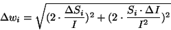 |
(4.4) |
where I is the total intensity as measured through ISOCAM's entrance
hole,  is its standard deviation and
  is the
standard deviation of the three polariser intensities.
is the
standard deviation of the three polariser intensities.
We define the corrected intensities as:
 |
(4.5) |
The best measure of the instrumental polarisation is given by CAM05
raster observations on the zodiacal background. Assuming that the
zodiacal background is flat and unpolarised, it is natural that any
measured degree of polarisation should reflect the instrumental
polarisation of ISOCAM. For the zodiacal light, we therefore write
the Stokes parameters as:
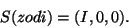 |
(4.6) |
The weight factors ( ) for all observed configurations are given
in Table 4.4. If one sets the polarisation
weight factors to unity, one derives from the zodiacal light images a
polarisation vector. Those vectors are given in
Table 4.5. They do not suggest a dependency on
wavelength nor on lens (pfov).
Already for the 3
) for all observed configurations are given
in Table 4.4. If one sets the polarisation
weight factors to unity, one derives from the zodiacal light images a
polarisation vector. Those vectors are given in
Table 4.5. They do not suggest a dependency on
wavelength nor on lens (pfov).
Already for the 3
 pfov the signal of the zodiacal
light tends to be weak and yields poor precision. For the
6
lens the mean instrumental polarisation is
around
pfov the signal of the zodiacal
light tends to be weak and yields poor precision. For the
6
lens the mean instrumental polarisation is
around  = 1.0
= 1.0 0.3%.
0.3%.
Table 4.4:
Polarisation weight factors  ,
,  normalised to
  = 1.
= 1.
|
Filter |
 |
lens |
|
 |
|
 |
| |
[ m] m] |
[
] |
|
[%] |
|
[%] |
|
LW2 |
6.7 |
6 |
0.9862 |
 0.1 0.1 |
0.9937 |
0.1 |
| LW10 |
12.0 |
6 |
0.9763 |
0.1 |
0.9926 |
0.1 |
| LW8 |
11.3 |
6 |
0.9829 |
0.1 |
0.9886 |
0.1 |
| LW3 |
14.3 |
6 |
0.9845 |
0.1 |
0.9937 |
0.1 |
| LW9 |
14.9 |
6 |
0.9873 |
0.1 |
0.9957 |
0.1 |
|
LW7 |
9.6 |
3 |
0.9824 |
2.1 |
0.9845 |
1.9 |
| LW8 |
11.3 |
3 |
0.9638 |
3.0 |
0.9740 |
3.0 |
| LW3 |
14.3 |
3 |
0.9614 |
0.4 |
0.9987 |
0.2 |
| LW9 |
14.9 |
3 |
0.9749 |
2.0 |
0.9865 |
2.2 |
|
LW3 |
14.3 |
1.5 |
0.9737 |
4.4 |
1.0022 |
4.2 |
Table 4.5:
Instrumental polarisation.
|
Filter |
|
lens |
|
 |
| |
[m] |
[
] |
[%] |
[ ] ] |
|
LW2 |
6.7 |
6 |
0.80 0.1 |
24 4 |
| LW10 |
12.0 |
6 |
1.41 0.1 |
29 3 |
| LW8 |
11.3 |
6 |
1.02 0.1 |
18 3 |
| LW3 |
14.3 |
6 |
0.91 0.1 |
26 3 |
| LW9 |
14.9 |
6 |
0.75 0.1 |
28 4 |
|
LW7 |
9.6 |
3 |
1.12 1.28 |
11 37 |
| LW8 |
11.3 |
3 |
2.20 2.05 |
16 27 |
| LW3 |
14.3 |
3 |
2.56 0.90 |
37 18 |
| LW9 |
14.9 |
3 |
1.47 1.47 |
22 27 |
|
LW3 |
14.3 |
1.5 |
1.85 3.3 |
40 38 |
The zodiacal light calibration observations give a good measure of
the LW flat-fields (Biviano et al. 1998c, [7]).
By combining the flat-fields
through the polarisers to calculate, for each detector element, a
Stokes vector, residual polarisation patterns can be noticed. There
is no strong dependency of the polarisation pattern on the filter. It
is quite similar for the 1.5
and
3
lens but shows a more aligned structure
using the 6
lens.
One corrects for this instrumental pattern in the
data by using the polarisation flat-fields. If such flat-fields cannot be
derived from one's own observation one may use those stored in the
calibration flat-field library. For a detailed description of CAM's
polarisation capabilities and how the instrumental polarisation was
determined see Siebenmorgen 1999, [55].
Next: 4.13 Global Error Budget
Up: 4. Calibration and Performance
Previous: 4.11 Astrometric Uncertainties
ISO Handbook Volume II (CAM), Version 2.0, SAI/1999-057/Dc