


An ISO observation is a combination of spacecraft and instrument operations. This section describes the available spacecraft observing modes and the overheads involved. An overhead is the time to prepare the satellite and instrument for a new observation or measurement before photons can be collected from the source.
In addition to the spacecraft observing modes the satellite construction constrains observations. The instruments are fixed with respect to the satellite axes (Figure 3.2). Therefore the satellite orientation determines how e.g. apertures are projected on the sky. This may be relevant when the aperture has a rectangular shape, when an array is used or when internal chopping was required. The instrument specific Handbooks provide detailed information about satellite orientation constraints.
The main operational mode of the spacecraft was a three-axis stabilised pointing at a target to carry out one or more observations, followed by a slew to another target.
A single pointing is an observation at a single sky position with a single instrument, which may consist of a series of measurements.
This was the standard mode used to observe `normal targets'
(i.e., point sources with fixed celestial coordinates). The
coordinate information had to be given with an accuracy of
1
![]() in
Declination and 0.1s in Right Ascension, the required accuracy at least
for the smaller entrance apertures of ISO. IRAS positions were thus
generally not precise enough for ISO. The instrument specific
volumes of the Handbook
describe problems encountered when observations were mispointed
(for various reasons).
in
Declination and 0.1s in Right Ascension, the required accuracy at least
for the smaller entrance apertures of ISO. IRAS positions were thus
generally not precise enough for ISO. The instrument specific
volumes of the Handbook
describe problems encountered when observations were mispointed
(for various reasons).
In order to avoid incorrect pointing, proper motion had to be given for objects such as nearby stars, in units of arcseconds per year.
Peaking-up was originally designed for observations which
require higher pointing accuracy, than the accuracy specified for the
spacecraft. Since the absolute pointing error (APE) was less than
2.5
![]() (see Section 5.4),
peaking-up was never used. This observing mode is here
included purely for historical reasons so that observers may understand the
term.
(see Section 5.4),
peaking-up was never used. This observing mode is here
included purely for historical reasons so that observers may understand the
term.
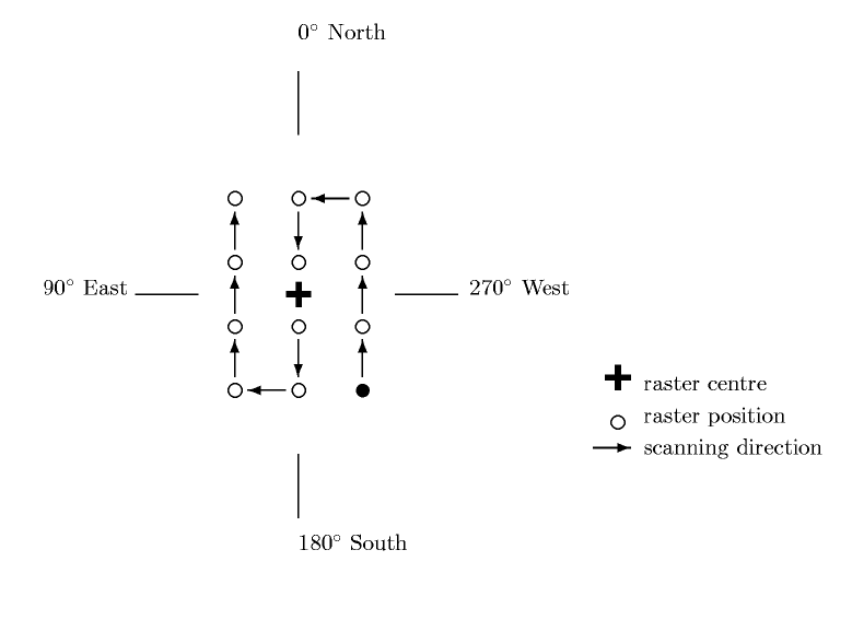
Spectroscopic and continuum maps could be obtained with a series of single pointings using the spacecraft raster mode. A map could contain one scan (one-dimensional mapping) or several scans (two-dimensional mapping). All pointings of a raster map had to lie within an area of 1.5 by 1.5 square degrees. Mapping was available for CAM, PHT and LWS. The observer had to specify the coordinates of the centre position, the number of scan lines (N), the number of points in a scan line (M) and the step sizes in arcseconds. The latter are the distance between the scan lines and the distance between points in the scan line. Additionally, the observer had to specify the position angle of the scan lines i.e. the orientation of the map (see Figures 4.9 and 4.10).
The number of points in a scanline and the number of scanlines can be any integer between 1 and 32. Setting one of the numbers to 1 specifies a one-dimensional scan. Allowed step sizes were 0,2,3,...,180 arcseconds.
A step size of 0
![]() in spacecraft z-direction was
used to simulate a `nodding' observation to achieve repeated
quasi-staring observations between target and one or more background
positions.
in spacecraft z-direction was
used to simulate a `nodding' observation to achieve repeated
quasi-staring observations between target and one or more background
positions.
The position entered into PGA for a raster map was taken as the center of the grid. Thus a 5 x 6 raster has its centre at, and therefore the position refers to, raster position (2.5,3).
The raster map parameters refer to:
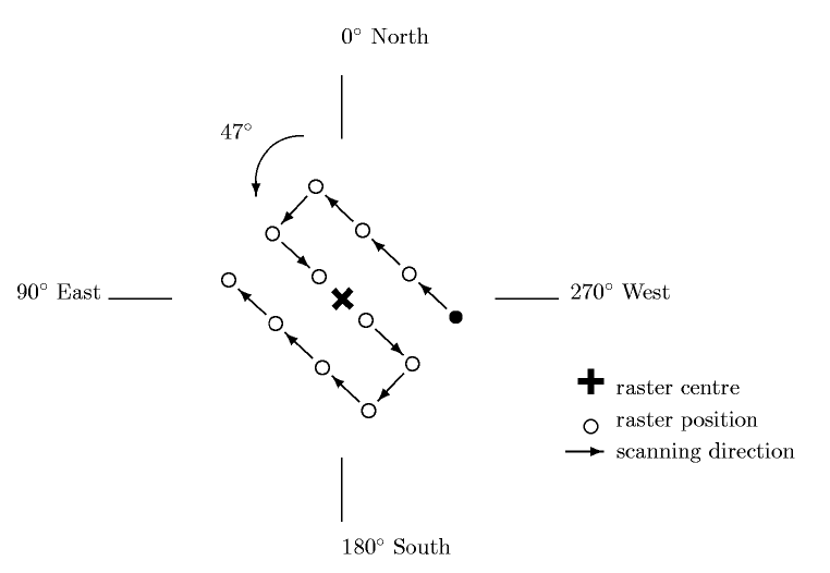
Figure 4.9 shows an example of an M=4, N=3 raster carried out with orientation angle=0, while Figure 4.10 shows one with an orientation angle of 47°.
Note that all angles are processed in J2000 coordinates.
|
|
The orientation angle of a map or a scan is counted from the North direction via East (see Figure 4.10). The values for the orientation angle can be between 0 and 179 degrees. A scan orientation angle of 90 degrees indicates that the scan was obtained going East-West. Note that the orientation angle, held for example in the IIPH keyword ATTRROTA, is different from the roll angle of the spacecraft, held for example in the IIPH keywords INSTROLL and CINSTROL. The roll angle indicates how the instrument apertures were placed on the sky and the orientation angle indicates how the raster was performed on the sky.
The map parameters are specified with respect to the equatorial coordinate system (Right Ascension and Declination for a given epoch). The orientation of the spacecraft axes was essentially arbitrary with respect to that system. Since the orientation of the detector arrays (i.e. CAM and PHT-C) and rectangular apertures (for PHT-P) is fixed with respect to the spacecraft axes, the orientation of the array or aperture with respect to the scan line was arbitrary. More details can be found in the CAM and PHT volumes of this Handbook. In some cases the spacecraft coordinate system was requested instead of the equatorial system to align the axes of a map with the spacecraft axes.
For scheduling, mapping was regarded as a single observation. Thus, a map, or a scan, was only scheduled as a whole or not at all.
Mapping was not available for SWS. There, maps were generated by concatenating individual observations together.
During pointings (both single pointings and raster pointings) the AOCS control about the spacecraft y- and z-axes was primarily achieved using the Star-Tracker. The control was to place the guide star on particular Star-Tracker `set-points' (which were calculated from the star vector, target quaternion and instrument alignments).
In raster mode the movement from one raster point to the next was simply achieved by appropriately changing the Star-Tracker set-points. This means the pointing accuracy of the first position of an M x N raster was set by the absolute pointing accuracy. The relative accuracy between any points in the raster is more difficult to determine. For rasters that did not move the star too much across the field of view of the Star-Tracker the pointing error should be of the order of the pointing jitter. However, for rasters that moved the star substantially across the field of view, the error could reach that of the APE, as the distortion might be different there.
Tracking of solar system objects was accomplished by using a 1-dimensional raster (effectively a time-dependent offset from background stars) and, therefore, raster pointing was not available to observers for designated solar system targets.
Concatenated observations are a chain of observations from the same proposal which had to be performed contiguously in time. All targets of the concatenated observations had to lie in an area of 3 degrees diameter.
For scheduling, concatenated observations were treated as a single unit, i.e. either all observations in the chain were scheduled or none. The underlying rationale for this treatment was that the proposer used concatenation to indicate that scheduling of only a part of these observations was not sufficient to meet the scientific objectives described in the proposal justification.
Note that concatenating observations simply because the pointings were close together in the sky was not a valid argument, since the mission planning system optimised the schedule very efficiently.
In principle up to 99 observations, the maximum allowed per proposal, could be concatenated. However, the more AOTs that were contained in the chain, the longer the duration of the entire observation; once this duration exceeded several hours, it became highly unlikely that the observation could be scheduled.
If carrying out an observation depends on the results of a previous observation, the corresponding two observations were called `linked'. The execution of these observations involved intervention by a resident astronomer, as the result of the first observation had to be evaluated on the basis of the specified observer requirements.
Examples of linked observations are:
A proposal requesting linked observations had to have a strong scientific case and to contain clear and quantitative specifications of the condition under which the later observation should be carried out. For scheduling reasons the later observations were carried out at least three revolutions later.
Archive users are unlikely to come across linked observations as the facility was rarely used during the mission.
Fixed time and periodic observations
Observations were carried out when they could be scheduled conveniently and without leading to large overheads, e.g. in target acquisition. Given the mission planning cycle, the time when an observation of a target would be scheduled was not known until the detailed schedule had been generated for a particular revolution a few days in advance.
However, there was the possibility to request an observation to be performed on a particular date (i.e. revolution) during the ISO mission. An example for this type of observing request is to observe a Mira variable at a certain phase in the light curve. The proposer specified in the scientific justification when the target was to be observed.
Periodic observations were a generalisation of fixed time observations. In the scientific justification, the proposer specified the date of the first observation, if e.g. the phase of the phenomenon to be observed was important. Additionally, the number of observations to be carried out and the number of days between successive observations had to be given. The small fraction of sky accessible from ISO at any given time rendered some periodic observations impossible.
These three special observing modes were used to make additional scientific observations either when the spacecraft was slewing to a new target or when CAM or LWS were not the prime instrument. These modes are the already mentioned:
These modes were not available to proposers, but the data is available in the ISO Data Archive.