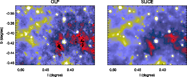
After the LTT has been corrected, we then take into account the
pixel-to-pixel temporal variations of the detector response. These
response variations (that
represent ![]() 1-3% of the average flat-field) are observed at various
time scales. To go further in the data processing, we try to correct these
pixel-to-pixel response variations with a time dependent flat-field
1-3% of the average flat-field) are observed at various
time scales. To go further in the data processing, we try to correct these
pixel-to-pixel response variations with a time dependent flat-field
![]() .
Flat-field and sky structures are mixed together in
.
Flat-field and sky structures are mixed together in
![]() (see Equation F.1) but the flat-field variations can be
extracted
from the data by estimating
(see Equation F.1) but the flat-field variations can be
extracted
from the data by estimating
![]() and by taking advantage of the
spatial redundancy.
and by taking advantage of the
spatial redundancy.
Here are the guidelines of this method:

|